Blog
2024-02-20
Back in November, I wrote about making 2n-page zines.
Thanks to some conversations I had at Big MathsJam
in later November, I've been able to work out how many 128-page zines there are: 315434.
The insight
At Big MathsJam, Colin Beveridge pointed out
something he'd noticed about the possible zines: when drawing the line connecting the pages
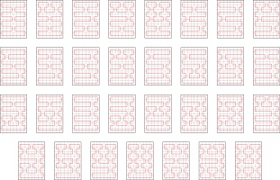
in order, there were some line segments that were always included. For example, here are all of the possible
64-page zines:
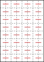
Every single one of these includes these line segments:
Colin conjectured that for a zine of any size, a pattern like this of alternative horizontal segments
must always be included. He was close to justifying this, and since MathsJam I've been able to fill
in the full justificication.
The justificiation
First, consider the left-most column of pages. They must be connected like this:
If they were connected in any other way, there would be two vertical connections in a row,
which would create a page that is impossible to open (as every other connection must be a horizontal
that ends up in the spine). Additionally, the horizontal lines in this diagram must all be in the
spine (as otherwise we again get pages that cannot be opened).
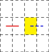
Next, consider a horizontal line that's in the spine (shown in red below), and we can look
at all the possible ways to draw the line through the highlighted page, paying particular
attention to the dashed blue line:
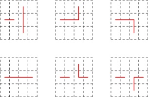
The six possible ways in which the line could travel through the highlighted page are:
The three options in the top row do not give a valid zine: the leftmost diagram has two vertical
connections in a row (leading to pages that do not open). The other two diagrams in the top row
have the horizontal line that we know is in the spine, followed by a horizontal line not in the
spine, then a vertial line: this vertical line should be in the spine, but as it is vertical
it cannot be (without making a page that doesn't open).
In each of the diagrams in the bottom row, the connection shown in dashed blue
is included and must be in the spine: in the leftmost diagram, the horizontal line that we know is in the spine
is followed by a horizontal not in the spine, then the horizinal in the dashed blue position
that must therefore be in the spine. The othe other two diagrams in the bottom row,
the dashed blue position is connected to a vertical line: this means that the dashed blue connection
must be in the spine (as otherwise the vertical would cause a page that doesn't open).
Overall, we've now shown that the leftmost column of lines must always be included and
must all be in the spine; and for each horizontal line in the spine, the line to the right of it
after a single gap must also be included and in the spine. From this, it follows that all the horizontal
lines in Colin's pattern must always be included.
Calculating the number of 128-page zines
Now that I knew that all these horizonal lines are always included, I was able to update
the code I was using to find all the possible zines
to use this. After a few hours, it had found all 315434 possibilites. I was very happy to get this
total, as it was the same as the number that
Luna (another attendee of Big MathsJam) had calculated but wasn't certain was correct.
The sequence of the number of 2n-page zines,
including the newly calculated number,
is now published on the OEIS.
I think calculating number of 256-page zines is still beyond my code though...
(Click on one of these icons to react to this blog post)
You might also enjoy...
Comments
Comments in green were written by me. Comments in blue were not written by me.
Add a Comment
2023-02-03
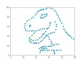
Imagine a set of 142 points on a two-dimensional graph.
The mean of the \(x\)-values of the points is 54.26.
The mean of the \(y\)-values of the points is 47.83.
The standard deviation of the \(x\)-values is 16.76.
The standard deviation of the \(y\)-values is 26.93.
What are you imagining that the data looks like?
Whatever you're thinking of, it's probably not this:
This is the datasaurus, a dataset that was created by Alberto Cairo in
2016 to remind people to look beyond the summary statistics when analysing a dataset.
Anscombe's quartet
In 1972, four datasets with a similar aim were publised. Graphs in statistical analysis by Francis J Anscombe [1] contained four datasets that have become known as Anscombe's quartet: they all have the same
mean \(x\)-value, mean \(y\)-value, standard deviation of \(x\)-values, standard deviation of \(y\)-values, linear regression line, as well multiple other values
related to correlation and variance. But if you plot them, the four datasets look very different:
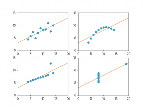
Plots of the four datasets that make up Anscombe's quartet. For each set of data:
the mean of the \(x\)-values is 9; the mean of the \(y\)-values is 7.5;
the standard deviation of the \(x\)-values is 3.32; the standard deviation of the \(y\)-values is 2.03;
the correlation coefficient between \(x\) and \(y\) is 0.816;
the linear regression line is \(y=3+0.5x\);
and coefficient of determination of linear regression is 0.667.
Anscombe noted that there were prevalent attitudes that:
- "Numerical calculations are exact, but graphs are rough."
- "For any particular kind of statistical data, there is just one set of calculations constituting a correct statistical analysis."
- "Performing intricate calculations is virtuous, actually looking at the data is cheating."
The four datasets were designed to counter these by showing that data exhibiting the same statistics can actually be very very different.
The datasaurus dozen
Anscombe's datasets indicate their point well, but the arrangement of the points is very regular and looks a little artificial when compared with real data sets.
In 2017, twelve sets of more realistic-looking data were published (in Same stats, different graphs: generating datasets with varied appearance and identical statistics through simulated annealing by Justin Matejka and George Fitzmaurice [2]).
These datasets—known as the datasaurus dozen—all had the same
mean \(x\)-value, mean \(y\)-value,
standard deviation of \(x\)-values, standard deviation of \(y\)-values, and corellation coefficient (to two decimal places) as the datasaurus.
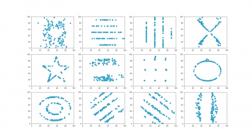
The twelve datasets that make up the datasaurus dozen. For each set of data (to two decimal places):
the mean of the \(x\)-values is 54.26; the mean of the \(y\)-values is 47.83;
the standard deviation of the \(x\)-values is 16.76; the standard deviation of the \(y\)-values is 26.93;
the correlation coefficient between \(x\) and \(y\) is -0.06.
Creating datasets like this is not trivial: if you have a set of values for the statistical properties of a dataset, it is difficult to create a dataset with those properties—especially
one that looks like a certain shape or pattern.
But if you already have one dataset with the desired properties, you can make other datasets with the same properties by very slightly moving every point in a random direction then
checking that the properties are the same—if you do this a few times, you'll eventually get a second dataset with the right properties.
The datasets in the datasaurus dozen were generated using this method: repeatedly adjusting all the points ever so slightly, checking if the properties were the same, then
keeping the updated data if it's closer to a target shape.
The databet
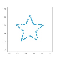
Using the same method, I generated the databet: a collection of datasets that look like the letters of the alphabet. I started with this set
of 100 points resembling a star:
After a long time repeatedly moving points by a very small amount, my computer eventually generated these 26 datasets, all of which have the same means,
standard deviations, and correlation coefficient:
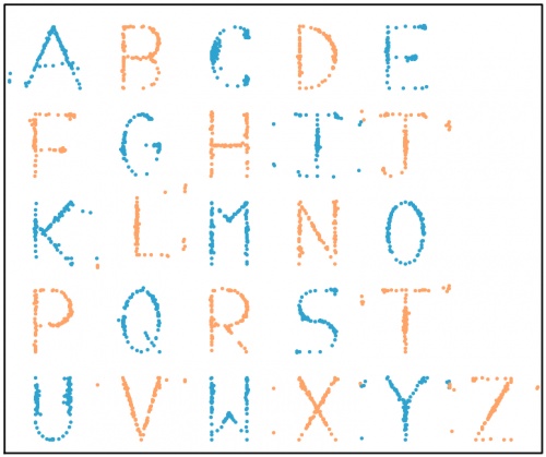
The databet. For each set of data (to two decimal places):
the mean of the \(x\)-values is 0.50; the mean of the \(y\)-values is 0.52;
the standard deviation of the \(x\)-values is 0.17; the standard deviation of the \(y\)-values is 0.18;
the correlation coefficient between \(x\) and \(y\) is 0.16.
Words
Now that we have the alphabet, we can write words using the databet. You can enter a word or phrase here to do this:
Given two data sets with the same number of points, we can make a new larger dataset by including all the points in both the smaller sets.
It is possible to write the mean and standard deviation of the larger dataset in terms of the means and standard deviations of the smaller sets: in each case,
the statistic of the larger set depends only on the statistics of the smaller sets and not on the actual data.
Applying this to the databet, we see that the datasets that spell words of a fixed length will all have the same mean and standard deviation.
(The same is not true, sadly, for the correlation coefficient.) For example, the datasets shown in the following plot both have the same means and standard deviations:
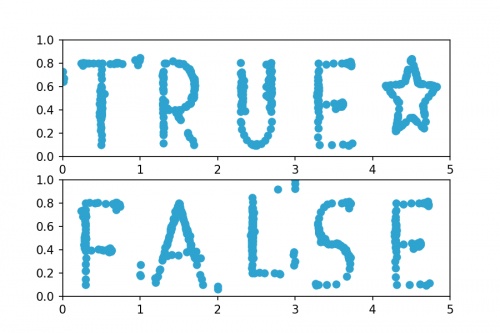
Datasets that spell "TRUE☆" and "FALSE". For both sets of (to two decimal places):
the mean of the \(x\)-values is 2.50; the mean of the \(y\)-values is 0.52;
the standard deviation of the \(x\)-values is 1.42; the standard deviation of the \(y\)-values is 0.18.
Hopefully by now you agree with me that Anscombe was right: it's very important to plot data as well as looking at the summary statistics.
If you want to play with the databet yourself, all the letters are available on GitHub in JSON format.
The GitHub repo also includes fonts that you can download and install so you can use Databet Sans in
your next important document.
References
[1] Graphs in statistical analysis by Francis J Anscombe. American Statistician, 1973.
[2] Same stats, different graphs: generating datasets with varied appearance and identical statistics through simulated annealing by Justin Matejka and George Fitzmaurice. Proceedings of the 2017 CHI Conference on Human Factors in Computing Systems, 2017.
(Click on one of these icons to react to this blog post)
You might also enjoy...
Comments
Comments in green were written by me. Comments in blue were not written by me.
Add a Comment
2022-02-26
Surprisingly often, people ask me how they can build their own copy of MENACE. If you've been thinking that you'd love your own matchbox-powered machine learning computer but haven't got round to asking me about it yet, then this blog post is just what you're looking for.
Matchboxes
Before building MENACE, you'll need to get hold of 304 matchboxes (plus a few spares in case one gets lost or falls apart). I used these craft matchboxes: they don't have the best build quality, but they're good enough.
304 positions
The positions you need to glue onto the front of the matchboxes can be downloaded from this GitHub repository (first move boxes, third move boxes, fifth move boxes, seventh move boxes). These are sized to fit on matchboxes that have 15mm by 35mm fronts.
I printed each pdf on differently coloured paper to make it easier to sort the matchboxes after getting them out of their box.
If you get differently sized matchboxes, the code used the generate the PDFs is in the same GitHub repository (you'll need to modify these lines). Alternatively, feel free to drop me an email and I will happily adjust the sizes for you and send you the updated PDFs.
Glue
I used PVA glue to stick the positions onto the matchboxes. The printable PDFs have extra tabs of paper above and below the postions that can be glued in to the bottom and inside of the matchbox tray to hold it more securely.
Gluing the positions onto the matchboxes was the most time consuming part of building my copy of MENACE, largely due to having to wait for the glue to dry on a set of matchboxes before I had space for the next batch of them to dry.
Beads
Once you've glued pictures of noughts and crosses positions to 304 matchboxes, you'll need to put coloured beads into each matchbox. For this, I used a large tub of Hama beads (that tub contained orders of magnitude more beads than I needed).
A nice side effect of using Hama beads is that they're designed to be ironed together so making a key to show which colour corresponds to each position is very easy.
I typically start the boxes off with 8 beads of each colour in the first move box, 4 of each colour in the third move boxes, 2 of each in the fifth move boxes, and one of each in the seventh move boxes.
Once you've filled all your matchboxes with the correct number of beads, you're ready to play yout first game against MENACE. I'd love to hear how you get on.
And once you're bored of playing noughts and crosses against your matchboxes, why not build a machine that learns to play Hexapawn, Connect 4, Chess or Go? Or one that plays Nim?
Edit: Added link to the printable pdfs of the positions needed for Hexapawn, made by Dan Whitman.
(Click on one of these icons to react to this blog post)
You might also enjoy...
Comments
Comments in green were written by me. Comments in blue were not written by me.
Interesting.
Could try a same kind of thing using playing card deck(s)? A(=1)-2-3 4-5-6 7-8-9 maybe 3 decks with different colours on their backs.
Could try a same kind of thing using playing card deck(s)? A(=1)-2-3 4-5-6 7-8-9 maybe 3 decks with different colours on their backs.
Willem
I also read the Martin Gardner article way back when and had two matchbox machines (actually with envelopes instead of matchboxes) play Nim against each other. I don't remember all the details now, except that it got to the point where one would make the first move and the other would immediately resign.
Tim Lewis
I made a matchbox machine that learns to play 3x3 Nim almost 50 years ago. I still have it. (Based on Martin Gardner's article)
Tony
Add a Comment
2019-06-19

A308092 The sum of the first \(n\) terms of the sequence is the concatenation of the first \(n\) bits of the sequence read as binary, with \(a(1) = 1\).1, 2, 3, 7, 14, 28, 56, 112, 224, 448, 896, 1791, 3583, 7166, ...

To understand this definition, let's look at the first few terms of this sequence written in binary:
By "the concatenation of the first \(n\) bits of the sequence", it means the first \(n\) binary digits of the whole sequence written in order:
1, then 11, then 110, then 1101, then 11011, then 110111, and so on. So the definition means:
- The first term is 1, as given in the definition (\(a(1)=1\)).
- The sum of the first 2 terms is the first 2 digits: \(1+10=11\).
- The sum of the first 3 terms is the first 3 digits: \(1+10+11=110\).
- The sum of the first 4 terms is the first 4 digits: \(1+10+11+111=1101\).
- The sum of the first 5 terms is the first 5 digits: \(1+10+11+111+1110=11011\).
As we know that the sum of the first \(n-1\) terms is the first \(n-1\) digits, we can calculate the third term of this sequence onwards using:
"\(a(n)\) is the concatenation of the first \(n\) bits of the sequence subtract concatenation of the first \(n-1\) bits of the sequence":
- The third term is \(110 - 11 = 11\).
- The fourth term is \(1101 - 110 = 111\).
- The fourth term is \(11011 - 1101 = 1110\).
- The fifth term is \(110111 - 11011 = 11100\).
The conjecture
Peter's conjecture is that the number of 1s in each term is greater than or equal to the number of 1s in the previous term.
I'm going to prove this conjecture. If you'd like to have a try first, stop reading now and come back when you're ready for spoilers.
(If you'd like a hint, read the next section then pause again.)
Adding a digit
The third term of the sequence onwards can be calculated by subtracting the first \(n-1\) digits from the first \(n\) digits.
If the first \(n-1\) digits form a binary number \(x\), then the first \(n\) digits will be \(2x+d\), where \(d\) is the \(n\)th digit
(because moving all the digits to the left one place in binary is multiplying by two).
Therefore the different is \(2x+d-x=x+d\), and so we can work out the \(n\)th term of the sequence by adding the \(n\)th digit in the
sequence to the first \(n-1\) digits. (Hat tip to Martin Harris, who spotted this first.)
Carrying
Adding 1 to a binary number the ends in 1 will cause 1 to carry over to the left. This carrying will continue until the 1 is carried into
a position containing 0, and after this all the digits to the left of this 0 will remain unchanged.
Therefore adding a digit to
the first \(n-1\) digits can only change the digits from the rightmost 0 onwards.
Endings
We can therefore disregard all the digits before the rightmost 0, and look at how the \(n\)th term compares to the \((n-1)\)th term.
There are 5 ways in which the first \(n\) digits could end:
- \(00\)
- \(010\)
- \(01...10\) (where \(1...1\) is a string of 2 or more ones)
- \(01\)
- \(01...1\) (where \(1...1\) is again a string of 2 or more ones)
We now look at each of these in turn and show that the \(n\)th term will contain at least as many ones at the \((n-1)\)th term.
Case 1: \(00\)
If the first \(n\) digits of the sequence are \(x00\) (a binary number \(x\) followed by two zeros), then the \((n-1)\)th term of the
sequence is \(x+0=x\), and the \(n\)th term of the sequence is \(x0+0=x0\). Both \(x\) and \(x0\) contain the same number of ones.
Case 2: \(010\)
If the first \(n\) digits of the sequence are \(x010\), then the \((n-1)\)th term of the sequence is \(x0+1=x1\),
and the \(n\)th term of the sequence is \(x01+0=x01\). Both \(x1\) and \(x01\) contain the same number of ones.
Case 3: \(01...10\)
If the first \(n\) digits of the sequence are \(x01...10\), then the \((n-1)\)th term of the sequence is \(x01...1+1=x10...0\),
and the \(n\)th term of the sequence is \(x01...10+1=x01...1\). \(x01...1\) contains more ones than \(x10...0\).
Case 4: \(01\)
If the first \(n\) digits of the sequence are \(x01\), then the \((n-1)\)th term of the sequence is \(x+0=x\),
and the \(n\)th term of the sequence is \(x0+1=x1\). \(x1\) contains one more one than \(x\).
Case 5: \(01...1\)
If the first \(n\) digits of the sequence are \(x01...1\), then the \((n-1)\)th term of the sequence is \(x01...1+1=x10...0\),
and the \(n\)th term of the sequence is \(x01...1+1=x10...0\). Both these contain the same number of ones.
In all five cases, the \(n\)th term contains more ones or an equal number of ones to the \((n-1)\)th term, and so the conjecture is true.
(Click on one of these icons to react to this blog post)
You might also enjoy...
Comments
Comments in green were written by me. Comments in blue were not written by me.
Add a Comment
2018-07-06
This is a post I wrote for round 1 of The Aperiodical's Big Internet Math-Off 2018, where Mathsteroids lost to MENACE.
A map projection is a way of representing the surface of a sphere, such as the Earth, on a flat surface. There is no way to represent all the features of a sphere on a flat surface, so if you want a map that shows a certain feature of the world, then you map will have to lose some other feature of the world in return.
To show you what different map projections do to a sphere, I have created a version of the game Asteroids on a sphere. I call it Mathsteroids. You can play it here, or follow the links below to play on specific projections.
Mercator projection
The most commonly used map projection is the Mercator projection, invented by Gerardus Mercator in 1569. The Mercator projection preserves angles: if two straight lines meet at an angle \(\theta\) on a sphere, then they will also meet at an angle \(\theta\) on the map. Keeping the angles the same, however, will cause the straight lines to no longer appear straight on the map, and the size of the same object in two different place to be very different.
The angle preserving property means that lines on a constant bearing (eg 030° from North) will appear straight on the map. These constant bearing lines are not actually straight lines on the sphere, but when your ship is already being buffeted about by the wind, the waves, and the whims of drunken sailors, a reasonably straight line is the best you can expect.
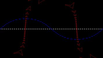
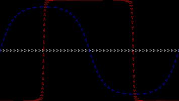
The picture below shows what three ships travelling in straight lines on the sphere look like on a Mercator projection.
To fully experience the Mercator projection, you can play Mathsteroids in Mercator projection mode here. Try flying North to see your spaceship become huge and distorted.
Gall–Peters projection
The Gall–Peters projection (named after James Gall and Arno Peters) is an area-preserving projection: objects on the map will have the same area as objects on the sphere, although the shape of the object on the projection can be very different to its shape on the sphere.
The picture below shows what three spaceships travelling in straight lines on a sphere look like on the Gall–Peters projection.
You can play Mathsteroids in Gall–Peters projection mode here. I find this one much harder to play than the Mercator projection, as the direction you're travelling changes in a strange way as you move.
Azimuthal projection
An azimuthal projection makes a map on which the directions from the centre point to other points on the map are the same as the directions on the sphere. A map like this could be useful if, for example, you're a radio operator and need to quickly see which direction you should point your aerial to communicate with other points on the map.
The azimuthal projection I've used in Mathsteroids also preserves distances: the distance from the centre to the another points on the map is proportional to the actual distance on the sphere. This projection is used as the emblem of the UN.
The picture below shows three straight lines on this projection. You can play Mathsteroids in azimuthal mode here.
A retroazimuthal projection makes a map on which the directions to the centre point from other points on the map are the same as the directions on the sphere. If you're thinking that this is the same as the azimuthal projection, then you're too used to doing geometry on flat surfaces: on a sphere, the sum of the angles in a triangle depends on the size of the triangle, so the directions from A to B and from B to A aren't as closely related as you would expect.
The Craig retroazimuthal projection was invented by James Ireland Craig in 1909. He used Mecca as his centre point to make a map that shows muslims across the world which direction they should face to pray.
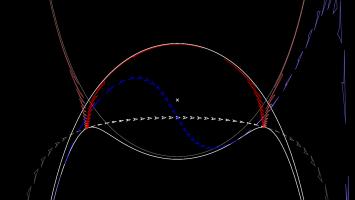
The picture below shows what three spaceships travelling in a straight lines on a sphere looks like on this projection.
You can play Mathsteroids in Craig retroazimuthal mode here to explore the projection yourself. This is perhaps the hardest of all to play, as (a) two different parts of the sphere overlap on the map, and (b) the map is actually infinitely tall, so quite a bit of it is off the edge of the visible game area.
Stereographic projection
The final projection I'd like to show you is the stereographic projection.
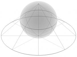
Imagine that a sphere is sitting on a 2D plane. Take a point on the sphere. Imagine a straight line through this point and the point at the top of the sphere. The point where this line meets the 2D plane is stereographic projection of the point on the sphere.
This projection (backwards) can be used to represent the every complex number as a point on a sphere: this is called the Riemann sphere.
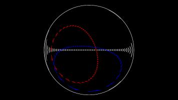
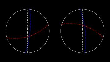
To make Mathseteroids playable after this projection, I split the sphere into 2 hemisphere and projected each seperately to give two circles. You can play Mathsteroids in stereographic projection mode here. Three spaceships travelling in straight lines on this projection are shown below.
... and if you still don't like map projections, you can still enjoy playing Mathsteroids on an old fashioned torus. Or on a Klein bottle or the real projective plane. Don't forget to take a short break from playing to head over to The Aperiodical and vote (voting now closed).
(Click on one of these icons to react to this blog post)
You might also enjoy...
Comments
Comments in green were written by me. Comments in blue were not written by me.
Add a Comment

