Blog
2019-07-03
This year's Big Internet Math-Off
is now underway with 15 completely new contestants (plus one returning contender). As I'm not the returning contestant, I haven't been spending
my time preparing my pitches. Instead, I've spent my time making an
unofficial Big Internet Math-Off sticker book.
To complete the sticker book, you will need to collect 162 different stickers. Every day, you will be given a pack of 5 stickers; there are
also some bonus packs available if you can find them (Hint: keep reading).
How many stickers will I need?
Using the same method as I did for last year's World Cup sticker book,
you can work out that the expected number of stickers needed to finish the sticker book:
If you have already stuck \(n\) stickers into your album, then the probability that the next sticker you get is new is
$$\frac{162-n}{162}.$$
The probability that the second sticker you get is the next new sticker is
$$\mathbb{P}(\text{next sticker is not new})\times\mathbb{P}(\text{sticker after next is new})$$
$$=\frac{n}{162}\times\frac{162-n}{162}.$$
Following the same method, we can see that the probability that the \(i\)th sticker you buy is the next new sticker is
$$\left(\frac{n}{162}\right)^{i-1}\times\frac{162-n}{162}.$$
Using this, we can calculate the expected number of stickers you will need to buy until you find a new one:
$$\sum_{i=1}^{\infty}i \left(\frac{162-n}{162}\right) \left(\frac{n}{162}\right)^{i-1} = \frac{162}{162-n}$$
Therefore, to get all 162 stickers, you should expect to buy
$$\sum_{n=0}^{161}\frac{162}{162-n} = 918 \text{ stickers}.$$
Using just your daily packs, it will take you until the end of the year to collect this many stickers.
Of course, you'll only need to collect this many if you don't swap your duplicate stickers.
How many stickers will I need if I swap?
To work out the expected number of stickers stickers you'd need if you swap, let's first think about two people who want to complete
their stickerbooks together. If there are \(a\) stickers that both collectors need and \(b\) stickers that one collector has and the other one
needs, then let \(E_{a,b}\) be the expected number of stickers they need to finish their sticker books.
The next sticker they get could be one of three things:
- A sticker they both need (with probability \(\frac{a}{162}\));
- A sticker one of them needs (with probability \(\frac{b}{162}\));
- A sticker they both have (with probability \(\frac{162-a-b}{162}\)).
Therefore, the expected number of stickers they need to complete their sticker books is
$$E_{a,b}=1+\frac{a}{162}E_{a-1,b+1}+\frac{b}{162}E_{a,b-1}+\frac{162-a-b}{162}E_{a,b}.$$
This can be rearranged to give
$$E_{a,b}=
\frac{162}{a+b}+
\frac{a}{a+b}E_{a-1,b+1}
+\frac{b}{a+b}E_{a,b-1}
$$
We know that $E_{0,0}=0$ (as if \(a=0\) and \(b=0\), both collectors have already finished their sticker books). Using this and the
formula above, we can work out that
$$E_{0,1}=162+E_{0,0}=162$$
$$E_{1,0}=162+E_{0,1}=324$$
$$E_{0,2}=\frac{162}2+E_{0,1}=243$$
$$E_{1,1}=\frac{162}2+\frac12E_{0,2}+\frac12E_{1,0}=364.5$$
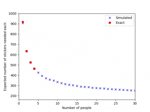
... and so on until we find that \(E_{162,0}=1269\), and so our collectors should expect to collect 634 stickers each to complete their
sticker books.
For three people, we can work out that if there are \(a\) stickers that all three need, \(b\) stickers that two need, and \(c\) stickers
that one needs, then
$$
E_{a,b,c}
= \frac{162}{a+b+c}+
\frac{a}{a+b+c}E_{a-1,b+1,c}
+\frac{b}{a+b+c}E_{a,b-1,c+1}
+\frac{c}{a+b+c}E_{a,b,c-1}.
$$
In the same way as for two people, we find that \(E_{162,0,0}=1572\), and so our collectors should expect to collect 524 stickers each
to complete their sticker books.
Doing the same thing for four people gives an expected 463 stickers required each.
After four people, however, the Python code I wrote to do these calculations takes too long to run, so instead I approximated the numbers
by simulating 500 groups of \(n\) people collecting stickers, and taking the average number of stickers they needed. The results are shown in
the graph below.
The red dots are the expected values we calculated exactly, and the blue crosses are the simulated values.
It looks like you'll need to collect at least 250 stickers to finish the album: in order to get this many before the end of the Math-Off,
you'll need to find 20 bonus packs...
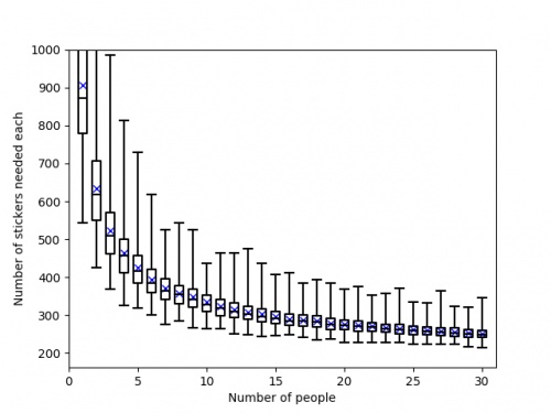
Of course, these are just the mean values and you could get lucky and need fewer stickers. The next graph shows box plots with the
quartiles of the data from the simulations.
So if you're lucky, you could complete the album with fewer stickers or fewer friends.
As a thank you for reading to the end of this blog post, here's a link that
will give you two bonus packs and help you on your way to the 250 expected stickers...
(Click on one of these icons to react to this blog post)
You might also enjoy...
Comments
Comments in green were written by me. Comments in blue were not written by me.
2019-07-06
@Pat Ashforth: Thanks, fixedMatthew
Link to sticker book, in the first paragraph, does not work. It points to mathoffstickbook.com
Pat Ashforth
minor typo for the 2 collector case
> and so our collectors should expect to collect 364 stickers
should be 634.
> and so our collectors should expect to collect 364 stickers
should be 634.
Road
Add a Comment


