Blog
PhD thesis, chapter 4
2020-02-13
This is the fourth post in a series of posts about my PhD thesis.
The fourth chapter of my thesis looks at weakly imposing Signorini boundary conditions on the boundary element method.
Signorini conditions
Signorini boundary conditions are composed of the following three conditions on the boundary:
\begin{align*}
u &\leqslant g\\
\frac{\partial u}{\partial n} &\leqslant \psi\\
\left(\frac{\partial u}{\partial n} -\psi\right)(u-g) &=0
\end{align*}
In these equations, \(u\) is the solution, \(\frac{\partial u}{\partial n}\) is the derivative of the solution in the direction normal to the boundary, and
\(g\) and \(\psi\) are (known) functions.
These conditions model an object that is coming into contact with a surface: imagine an object that is being pushed upwards towards a surface. \(u\) is the height of the object at
each point; \(\frac{\partial u}{\partial n}\) is the speed the object is moving upwards at each point; \(g\) is the height of the surface; and \(\psi\) is the speed at which the upwards force will cause
the object to move. We now consider the meaning of each of the three conditions.
The first condition (\(u \leqslant g\) says the the height of the object is less than or equal to the height of the surface. Or in other words, no part of the object has been pushed through
the surface. If you've ever picked up a real object, you will see that this is sensible.
The second condition (\(\frac{\partial u}{\partial n} \leqslant \psi\)) says that the speed of the object is less than or equal to the speed that the upwards force will cause. Or in other words,
the is no extra hidden force that could cause the object to move faster.
The final condition (\(\left(\frac{\partial u}{\partial n} -\psi\right)(u-g)=0\)) says that either \(u=g\) or \(\frac{\partial u}{\partial n}=\psi\). Or in other words, either the object is touching
the surface, or it is not and so it is travelling at the speed caused by the force.
Non-linear problems
It is possible to rewrite these conditions as the following, where \(c\) is any positive constant:
$$u-g=\left[u-g + c\left(\frac{\partial u}{\partial n}-\psi\right)\right]_-$$
The term \(\left[a\right]_-\) is equal to \(a\) if \(a\) is negative or 0 if \(a\) is positive (ie \(\left[a\right]_-=\min(0,a)\)).
If you think about what this will be equal to if \(u=g\), \(u\lt g\), \(\frac{\partial u}{\partial n}=\psi\), and \(\frac{\partial u}{\partial n}\lt\psi\), you can convince yourself
that it is equivalent to the three Signorini conditions.
Writing the condition like this is helpful, as this can easily be added into the matrix system due to the boundary element method to weakly impose it. There is, however, a complication:
due to the \([\cdot]_-\) operator, the term we add on is non-linear and cannot be represented as a matrix. We therefore need to do a little more than simply use our favourite
matrix solver to solve this problem.
To solve this non-linear system, we use an iterative approach: first make a guess at what the solution might be (eg guess that \(u=0\)). We then use this guess to calculate the value
of the non-linear term, then solve the linear system obtained when the value is substituted in. This gives us a second guess of the solution: we can do follow the same approach to obtain a third
guess. And a fourth. And a fifth. We continue until one of our guesses is very close to the following guess, and we have an approximation of the solution.
Analysis
After deriving formulations for weakly imposed Signorini conditions on the boundary element method, we proceed as we did in chapter 3 and analyse the method.
The analysis in chapter 4 differs from that in chapter 3 as the system in this chapter is non-linear. The final result, however, closely resembles the results in chapter 3: we obtain
and a priori error bounds:
$$\left\|u-u_h\right\|\leqslant ch^{a}\left\|u\right\|$$
As in chapter 3, The value of the constant \(a\) for the spaces we use is \(\tfrac32\).
Numerical results
As in chapter 3, we used Bempp to run some numerical experiments to demonstrate the performance of this method.

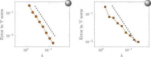
The error of our approximate solutions of a Signorini problem on the interior of a sphere with meshes with different values of \(h\) for two choices of combinations of discrete spaces. The
dashed lines show order \(\tfrac32\) convergence.
These results are for two different combinations of the discrete spaces we looked at in chapter 2. The plot on the left shows the expected
order \(\tfrac32\). The plot on the right, however, shows a lower convergence than our a priori error bound predicted. This is due to the matrices obtained when using this combination of spaces
being ill-conditioned, and so our solver struggles to find a good solution. This ill-conditioning is worse for smaller values of \(h\), which is
why the plot starts at around the expected order of convergence, but then the convergence tails off.
These results conclude chapter 4 of my thesis.
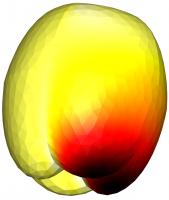
Why not take a break and snack on the following figure before reading on.

The solution of a mixed Dirichlet–Signorini problem on the interior of an apple, solved using weakly imposed boundary conditions.
Previous post in series
This is the fourth post in a series of posts about my PhD thesis.
Next post in series
(Click on one of these icons to react to this blog post)
You might also enjoy...
Comments
Comments in green were written by me. Comments in blue were not written by me.
Add a Comment


