
Blog
PhD thesis, chapter 3
2020-02-11
This is the third post in a series of posts about my PhD thesis.
In the third chapter of my thesis, we look at how boundary conditions can be weakly imposed when using the boundary element method.
Weak imposition of boundary condition is a fairly popular approach when using the finite element method, but our application of it to the boundary element method, and our analysis of
it, is new.
But before we can look at this, we must first look at what boundary conditions are and what weak imposition means.
Boundary conditions
A boundary condition comes alongside the PDE as part of the problem we are trying to solve. As the name suggests, it is a condition on the boundary: it tells us what the
solution to the problem will do at the edge of the region we are solving the problem in. For example, if we are solving a problem involving sound waves hitting an object, the
boundary condition could tell us that the object reflects all the sound, or absorbs all the sound, or does something inbetween these two.
The most commonly used boundary conditions are Dirichlet conditions, Neumann conditions and Robin conditions.
Dirichlet conditions say that the solution has a certain value on the boundary;
Neumann conditions say that derivative of the solution has a certain value on the boundary;
Robin conditions say that the solution at its derivate are in some way related to each other (eg one is two times the other).
Imposing boundary conditions
Without boundary conditions, the PDE will have many solutions. This is analagous to the following matrix problem, or the equivalent system of simultaneous equations.
\begin{align*}
\begin{bmatrix}
1&2&0\\
3&1&1\\
4&3&1
\end{bmatrix}\mathbf{x}
&=
\begin{pmatrix}
3\\4\\7
\end{pmatrix}
&&\text{or}&
\begin{array}{3}
&1x+2y+0z=3\\
&3x+1y+1z=4\\
&4x+3y+1z=7
\end{array}
\end{align*}
This system has an infinite number of solutions: for any number \(a\), \(x=a\), \(y=\tfrac12(3-a)\), \(z=4-\tfrac52a-\tfrac32\) is a solution.
A boundary condition is analagous to adding an extra condition to give this system a unique solution, for example \(x=a=1\). The usual way of imposing
a boundary condition is to substitute the condition into our equations. In this example we would get:
\begin{align*}
\begin{bmatrix}
2&0\\
1&1\\
3&1
\end{bmatrix}\mathbf{y}
&=
\begin{pmatrix}
2\\1\\3
\end{pmatrix}
&&\text{or}&
\begin{array}{3}
&2y+0z=2\\
&1y+1z=1\\
&3y+1z=3
\end{array}
\end{align*}
We can then remove one of these equations to leave a square, invertible matrix. For example, dropping the middle equation gives:
\begin{align*}
\begin{bmatrix}
2&0\\
3&1
\end{bmatrix}\mathbf{y}
&=
\begin{pmatrix}
2\\3
\end{pmatrix}
&&\text{or}&
\begin{array}{3}
&2y+0z=2\\
&3y+1z=3
\end{array}
\end{align*}
This problem now has one unique solution (\(y=1\), \(z=0\)).
Weakly imposing boundary conditions
To weakly impose a boundary conditions, a different approach is taken: instead of substituting (for example) \(x=1\) into our system, we add \(x\) to one side of an equation
and we add \(1\) to the other side. Doing this to the first equation gives:
\begin{align*}
\begin{bmatrix}
2&2&0\\
3&1&1\\
4&3&1
\end{bmatrix}\mathbf{x}
&=
\begin{pmatrix}
4\\4\\7
\end{pmatrix}
&&\text{or}&
\begin{array}{3}
&2x+2y+0z=4\\
&3x+1y+1z=4\\
&4x+3y+1z=7
\end{array}
\end{align*}
This system now has one unique solution (\(x=1\), \(y=1\), \(z=0\)).
In this example, weakly imposing the boundary condition seems worse than substituting, as it leads to a larger problem which will take longer to solve.
This is true, but if you had a more complicated condition (eg \(\sin x=0.5\) or \(\max(x,y)=2\)), it is not always possible to write the condition in a nice way that can be substituted in,
but it is easy to weakly impose the condition (although the result will not always be a linear matrix system, but more on that in chapter 4).
Analysis
In the third chapter of my thesis, we wrote out the derivations of formulations of the weak imposition of Dirichet, Neumann, mixed Dirichlet–Neumann, and Robin conditions on Laplace's equation:
we limited our work in this chapter to Laplace's equation as it is easier to analyse than the Helmholtz equation.
Once the formulations were derived, we proved some results about them: the main result that this analysis leads to is the proof of a priori error bounds.
An a priori error bound tells you how big the difference between your approximation and the actual solution will be.
These bounds are called a priori as they can be calculated before you solve the problem (as opposed to a posteriori error bounds that are calculated after solving the problem
to give you an idea of how accurate you are and which parts of the solution are more or less accurate).
Proving these bounds is important, as proving this kind of bound shows that your method will give a good approximation of the actual solution.
A priori error bounds look like this:
$$\left\|u-u_h\right\|\leqslant ch^{a}\left\|u\right\|$$
In this equation, \(u\) is the solution of the actual PDE problem; \(u_h\) is our appoximation; the \(h\) that appears in \(u_h\) and on the right-hand size is
the length of the longest edge in the mesh we are using; and \(c\) and \(a\) are positive constants. The vertical lines \(\|\cdot\|\) are a measurement of the size of a function.
Overall, the equation says that the size of the difference between the solution and our approximation (ie the error) is smaller than a constant times \(h^a\) times the size of
the solution. Because \(a\) is positive, \(h^a\) gets smaller as \(h\) get smaller, and so if we make the triangles in our mesh smaller (and so have more of them), we will see our error getting
smaller.
The value of the constant \(a\) depends on the choices of discretisation spaces used: using the spaces in the previous chapter gives \(a\) equal to \(\tfrac32\).
Numerical results
Using Bempp, we approximated the solution on a series of meshes with different values of \(h\) to check that we do indeed get order \(\tfrac32\) convergence.
By plotting \(\log\left(\left\|u-u_h\right\|\right)\) against \(\log h\), we obtain a graph with gradient \(a\) and can easily compare this gradient to a gradient of \(\tfrac32\).
Here are a couple of our results:
)
The errors of a Dirichlet problem on a cube (left) and a Robin problem on a sphere (right) as \(h\) is decreased. The dashed lines show order \(\tfrac32\) convergence.
Note that the \(\log h\) axis is reversed, as I find these plots easier to interpret this way found. Pleasingly, in these numerical experiments, the order of convergence agrees with
the a priori bounds that we proved in this chapter.
These results conclude chapter 3 of my thesis.
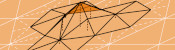
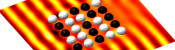
Why not take a break and refill the following figure with hot liquid before reading on.
)
The solution of a mixed Dirichlet–Neumann problem on the interior of a mug, solved using weakly imposed boundary conditions.
Previous post in series
This is the third post in a series of posts about my PhD thesis.
Next post in series

(Click on one of these icons to react to this blog post)
You might also enjoy...

Comments
Comments in green were written by me. Comments in blue were not written by me.
Add a Comment