Blog
Log-scaled axes
2020-03-31
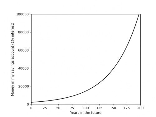
Recently, you've probably seen a lot of graphs that look like this:
The graph above shows something that is growing exponentially: its equation is \(y=kr^x\), for some constants \(k\) and \(r\).
The value of the constant \(r\) is very important, as it tells you how quickly the value is going to grow. Using a graph of some data,
it is difficult to get an anywhere-near-accurate approximation of \(r\).
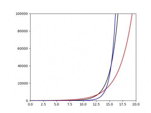
The following plot shows three different exponentials. It's very difficult to say anything about them except that they grow very quickly above around \(x=15\).
It would be nice if we could plot these in a way that their important properties—such as the value of the ratio \(r\)—were more clearly evident from the
graph. To do this, we start by taking the log of both sides of the equation:
$$\log y=\log(kr^x)$$
Using the laws of logs, this simplifies to:
$$\log y=\log k+x\log r$$
This is now the equation of a straight line, \(\hat{y}=m\hat{x}+c\), with \(\hat{y}=\log y\), \(\hat{x}=x\), \(m=\log r\) and \(c=\log k\). So if we plot
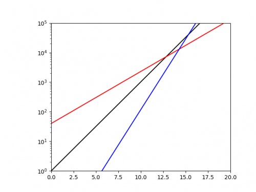
\(x\) against \(\log y\), we should get a straight line with gradient \(\log r\). If we plot the same three exponentials as above using a log-scaled \(y\)-axis, we get:
From this picture alone, it is very clear that the blue exponential has the largest value of \(r\), and we could quickly work out a decent approximation of this value
by calculating 10 (or the base of the log used if using a different log) to the power of the gradient.
Log-log plots
Exponential growth isn't the only situation where scaling the axes is beneficial. In my research in finite and boundary element methods,
it is common that the error of the solution \(e\) is given in terms of a grid parameter \(h\) by a polynomial of the form
\(e=ah^k\),
for some constants \(a\) and \(k\).
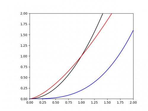
We are often interested in the value of the power \(k\). If we plot \(e\) against \(h\), it's once again difficult to judge the value of \(k\) from the graph alone. The following
graph shows three polynomials.
Once again is is difficult to judge any of the important properties of these. To improve this, we once again begin by taking the log of each side of the equation:
$$\log e=\log (ah^k)$$
Applying the laws of logs this time gives:
$$\log e=\log a+k\log h$$
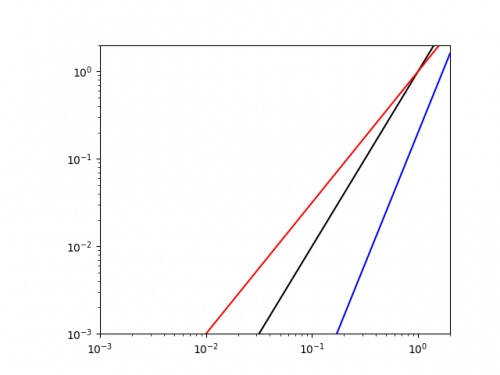
This is now the equation of a straight line, \(\hat{y}=m\hat{x}+c\), with \(\hat{y}=\log e\), \(\hat{x}=\log h\), \(m=k\) and \(c=\log a\). So if we plot
\(\log x\) against \(\log y\), we should get a straight line with gradient \(k\).
Doing this for the same three curves as above gives the following plot.
It is easy to see that the blue line has the highest value of \(k\) (as it has the highest gradient, and we could get a decent approximation of this value by finding the line's gradient.
As well as making it easier to get good approximations of important parameters, making curves into straight lines in this way also makes it easier to plot the trend of real data.
Drawing accurate exponentials and polynomials is hard at the best of times; and real data will not exactly follow the curve, so drawing an exponential or quadratic of best fit will be an
even harder task. By scaling the axes first though, this task simplifies to drawing a straight line through the data; this is much easier.
So next time you're struggling with an awkward curve, why not try turning it into a straight line first.
(Click on one of these icons to react to this blog post)
You might also enjoy...
Comments
Comments in green were written by me. Comments in blue were not written by me.
Add a Comment

