
Blog
2020-02-06
This is the third post in a series of posts about matrix methods.
Yet again, we want to solve \(\mathbf{A}\mathbf{x}=\mathbf{b}\), where \(\mathbf{A}\) is a (known) matrix, \(\mathbf{b}\) is a (known) vector, and \(\mathbf{x}\) is an unknown vector.
In the previous post in this series, we used Gaussian elimination to invert a matrix.
You may, however, have been taught an alternative method for calculating the inverse of a matrix. This method has four steps:
- Find the determinants of smaller blocks of the matrix to find the "matrix of minors".
- Multiply some of the entries by -1 to get the "matrix of cofactors".
- Transpose the matrix.
- Divide by the determinant of the matrix you started with.
An example
As an example, we will find the inverse of the following matrix.
$$\begin{pmatrix}
1&-2&4\\
-2&3&-2\\
-2&2&2
\end{pmatrix}.$$
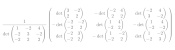
The result of the four steps above is the calculation
$$\frac1{\det\begin{pmatrix}
1&-2&4\\
-2&3&-2\\
-2&2&2
\end{pmatrix}
}\begin{pmatrix}
\det\begin{pmatrix}3&-2\\2&2\end{pmatrix}&
-\det\begin{pmatrix}-2&4\\2&2\end{pmatrix}&
\det\begin{pmatrix}-2&4\\3&-2\end{pmatrix}\\
-\det\begin{pmatrix}-2&-2\\-2&2\end{pmatrix}&
\det\begin{pmatrix}1&4\\-2&2\end{pmatrix}&
-\det\begin{pmatrix}1&4\\-2&-2\end{pmatrix}\\
\det\begin{pmatrix}-2&3\\-2&2\end{pmatrix}&
-\det\begin{pmatrix}1&-2\\-2&2\end{pmatrix}&
\det\begin{pmatrix}1&-2\\-2&3\end{pmatrix}
\end{pmatrix}.$$
Calculating the determinants gives
$$\frac12
\begin{pmatrix}
10&12&-8\\
8&10&-6\\
2&2&-1
\end{pmatrix},$$
which simplifies to
$$
\begin{pmatrix}
5&6&-4\\
4&5&-3\\
1&1&-\tfrac12
\end{pmatrix}.$$
How many operations
This method can be used to find the inverse of a matrix of any size. Using this method on an \(n\times n\) matrix will require:
- Finding the determinant of \(n^2\) different \((n-1)\times(n-1)\) matrices.
- Multiplying \(\left\lfloor\tfrac{n}2\right\rfloor\) of these matrices by -1.
- Calculating the determinant of a \(n\times n\) matrix.
- Dividing \(n^2\) numbers by this determinant.
If \(d_n\) is the number of operations needed to find the determinant of an \(n\times n\) matrix, the total number of operations for this method is
$$n^2d_{n-1} + \left\lfloor\tfrac{n}2\right\rfloor + d_n + n^2.$$
How many operations to find a determinant
If you work through the usual method of calculating the determinant by calculating determinants of smaller blocks the combining them, you
can work out that the number of operations needed to calculate a determinant in this way is \(\mathcal{O}(n!)\). For large values of \(n\), this is significantly larger than any power of \(n\).
There are other methods of calculating determinants: the fastest of these
is \(\mathcal{O}(n^{2.373})\). For large \(n\), this is significantly smaller than \(\mathcal{O}(n!)\).
How many operations
Even if the quick \(\mathcal{O}(n^{2.373})\) method for calculating determinants is used, the number of operations required to invert a matrix will be of the order of
$$n^2(n-1)^{2.373} + \left\lfloor\tfrac{n}2\right\rfloor + n^{2.373} + n^2.$$
This is \(\mathcal{O}(n^{4.373})\), and so for large matrices this will be slower than Gaussian elimination, which was \(\mathcal{O}(n^3)\).
In fact, this method could only be faster than Gaussian elimination if you discovered a method of finding a determinant faster than \(\mathcal{O}(n)\). This seems highly unlikely
to be possible, as an \(n\times n\) matrix has \(n^2\) entries and we should expect to operate on each of these at least once.
So, for large matrices, Gaussian elimination looks like it will always be faster, so you can safely forget this four-step method.
Previous post in series
This is the third post in a series of posts about matrix methods.
(Click on one of these icons to react to this blog post)
You might also enjoy...


Comments
Comments in green were written by me. Comments in blue were not written by me.
Add a Comment
2020-01-24
This is the second post in a series of posts about matrix methods.
We want to solve \(\mathbf{A}\mathbf{x}=\mathbf{b}\), where \(\mathbf{A}\) is a (known) matrix, \(\mathbf{b}\) is a (known) vector, and \(\mathbf{x}\) is an unknown vector.
This matrix system can be thought of as a way of representing simultaneous equations. For example, the following matrix problem and system of simultaneous equations are equivalent.
\begin{align*}
\begin{pmatrix}2&1\\3&1\end{pmatrix}\mathbf{x}&=\begin{pmatrix}3\\4\end{pmatrix}
&&\quad&&
\begin{array}{r}
2x+2y=3&\\
3x+2y=4&
\end{array}
\end{align*}
The simultaneous equations here would usually be solved by adding or subtracting the equations together. In this example, subtracting the first equation from the second gives \(x=1\).
From there, it is not hard to find that \(y=\frac12\).
One approach to solving \(\mathbf{A}\mathbf{x}=\mathbf{b}\) is to find the inverse matrix \(\mathbf{A}^{-1}\), and use \(\mathbf{x}=\mathbf{A}^{-1}\mathbf{b}\). In this post, we use Gaussian elimination—a method
that closely resembles the simultaneous equation method—to find \(\mathbf{A}^{-1}\).
Gaussian elimination
As an example, we will use Gaussian elimination to find the inverse of the matrix
$$\begin{pmatrix}
1&-2&4\\
-2&3&-2\\
-2&2&2
\end{pmatrix}.$$
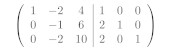
First, write the matrix with an identity matrix next to it.
$$\left(\begin{array}{ccc|ccc}
1&-2&4&1&0&0\\
-2&3&-2&0&1&0\\
-2&2&2&0&0&1
\end{array}\right)$$
Our aim is then to use row operations to change the matrix on the left of the vertical line into the identity matrix, as
the matrix on the right will then be the inverse. We are allowed to use two row operations: we can multiply a row by a scalar; or we can add a multiple of a row to another row.
These operations closely resemble the steps used to solve simultaneous equations.
We will get the matrix to the left of the vertical line to be the identity in a systematic manner: our first aim is to get the first column to read 1, 0, 0.
We already have the 1; to get the 0s, add 2 times the first row to both the second and third rows.
$$\left(\begin{array}{ccc|ccc}
1&-2&4&1&0&0\\
0&-1&6&2&1&0\\
0&-2&10&2&0&1
\end{array}\right)$$
Our next aim is to get the second column to read 0, 1, 0. To get the 1, we multiply the second row by -1.
$$\left(\begin{array}{ccc|ccc}
1&-2&4&1&0&0\\
0&1&-6&-2&-1&0\\
0&-2&10&2&0&1
\end{array}\right)$$
To get the 0s, we add 2 times the second row to both the first and third rows.
$$\left(\begin{array}{ccc|ccc}
1&0&-8&-3&-2&0\\
0&1&-6&-2&-1&0\\
0&0&-2&-2&-2&1
\end{array}\right)$$
Our final aim is to get the third column to read 0, 0, 1. To get the 1, we multiply the third row by -½.
$$\left(\begin{array}{ccc|ccc}
1&0&-8&-3&-2&0\\
0&1&-6&-2&-1&0\\
0&0&1&1&1&-\tfrac{1}{2}
\end{array}\right)$$
To get the 0s, we add 8 and 6 times the third row to the first and second rows (respectively).
$$\left(\begin{array}{ccc|ccc}
1&0&0&5&6&-4\\
0&1&0&4&5&-3\\
0&0&1&1&1&-\tfrac{1}{2}
\end{array}\right)$$
We have the identity on the left of the vertical bar, so we can conclude that
$$\begin{pmatrix}
1&-2&4\\
-2&3&-2\\
-2&2&2
\end{pmatrix}^{-1}
=
\begin{pmatrix}
5&6&-4\\
4&5&-3\\
1&1&-\tfrac{1}{2}
\end{pmatrix}.$$
How many operations
This method can be used on matrices of any size. We can imagine doing this with an \(n\times n\) matrix and look at how many operations
the method will require, as this will give us an idea of how long this method would take for very large matrices.
Here, we count each use of \(+\), \(-\), \(\times\) and \(\div\) as a (floating point) operation (often called a flop).
Let's think about what needs to be done to get the \(i\)th column of the matrix equal to 0, ..., 0, 1, 0, ..., 0.
First, we need to divide everything in the \(i\)th row by the value in the \(i\)th row and \(i\)th column. The first \(i-1\) entries in the column will already be 0s though, so there is no need to divide
these. This leaves \(n-(i-1)\) entries that need to be divided, so this step takes \(n-(i-1)\), or \(n+1-i\) operations.
Next, for each other row (let's call this the \(j\)th row), we add or subtract a multiple of the \(i\)th row from the \(j\)th row. (Again the first \(i-1\) entries can be ignored as they are 0.)
Multiplying the \(i\)th row takes \(n+1-i\) operations, then adding/subtracting takes another \(n+1-i\) operations.
This needs to be done for \(n-1\) rows, so takes a total of \(2(n-1)(n+1-i)\) operations.
After these two steps, we have finished with the \(i\)th column, in a total of \((2n-1)(n+1-i)\) operations.
We have to do this for each \(i\) from 1 to \(n\), so the total number of operations to complete Gaussian elimination is
$$
(2n-1)(n+1-1)
+
(2n-1)(n+1-2)
+...+
(2n-1)(n+1-n)
$$
This simplifies to
$$\tfrac12n(2n-1)(n+1)$$
or
$$n^3+\tfrac12n^2-\tfrac12n.$$
The highest power of \(n\) is \(n^3\), so we say that this algorithm is an order \(n^3\) algorithm, often written \(\mathcal{O}(n^3)\).
We focus on the highest power of \(n\) as if \(n\) is very large, \(n^3\) will be by far the largest number in the expression, so gives us an idea of how fast/slow this algorithm will be for large
matrices.
\(n^3\) is not a bad start—it's far better than \(n^4\), \(n^5\), or \(2^n\)—but there are methods out there that will take less than \(n^3\) operations.
We'll see some of these later in this series.
Previous post in series
This is the second post in a series of posts about matrix methods.
Next post in series
(Click on one of these icons to react to this blog post)
You might also enjoy...
Comments
Comments in green were written by me. Comments in blue were not written by me.
Add a Comment
2020-01-23
This is the first post in a series of posts about matrix methods.
When you first learn about matrices, you learn that in order to multiply two matrices, you use this strange-looking method involving the rows of the left matrix and the columns of this right.
)
It doesn't immediately seem clear why this should be the way to multiply matrices. In this blog post, we look at why this is the definition of matrix multiplication.
Simultaneous equations
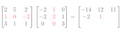
Matrices can be thought of as representing a system of simultaneous equations. For example, solving the matrix problem
$$
\begin{bmatrix}2&5&2\\1&0&-2\\3&1&1\end{bmatrix}
\begin{pmatrix}x\\y\\z\end{pmatrix}
=
\begin{pmatrix}14\\-16\\-4\end{pmatrix}
$$
is equivalent to solving the following simultaneous equations.
\begin{align*}
2x+5y+2z&=14\\
1x+0y-2z&=-16\\
3x+1y+1z&=-4
\end{align*}
Two matrices
Now, let \(\mathbf{A}\) and \(\mathbf{C}\) be two 3×3 matrices, let \(\mathbf{b}\) by a vector with three elements, and let \(\mathbf{x}=(x,y,z)\).
We consider the equation
$$\mathbf{A}\mathbf{C}\mathbf{x}=\mathbf{b}.$$
In order to understand what this equation means, we let \(\mathbf{y}=\mathbf{C}\mathbf{x}\) and think about solving the two simuntaneous matrix equations,
\begin{align*}
\mathbf{A}\mathbf{y}&=\mathbf{b}\\
\mathbf{C}\mathbf{x}&=\mathbf{y}.
\end{align*}
We can write the entries of \(\mathbf{A}\), \(\mathbf{C}\), \(\mathbf{x}\), \(\mathbf{y}\) and \(\mathbf{b}\) as
\begin{align*}
\mathbf{A}&=\begin{bmatrix}
a_{11}&a_{12}&a_{13}\\
a_{21}&a_{22}&a_{23}\\
a_{31}&a_{32}&a_{23}
\end{bmatrix}
&
\mathbf{C}&=\begin{bmatrix}
c_{11}&c_{12}&c_{13}\\
c_{21}&c_{22}&c_{23}\\
c_{31}&c_{32}&c_{23}
\end{bmatrix}
\end{align*}
\begin{align*}
\mathbf{x}&=\begin{pmatrix}x_1\\x_2\\x_3\end{pmatrix}
&
\mathbf{y}&=\begin{pmatrix}y_1\\y_2\\y_3\end{pmatrix}
&
\mathbf{b}&=\begin{pmatrix}b_1\\b_2\\b_3\end{pmatrix}
\end{align*}
We can then write out the simultaneous equations that \(\mathbf{A}\mathbf{y}=\mathbf{b}\) and \(\mathbf{C}\mathbf{x}=\mathbf{y}\) represent:
\begin{align}
a_{11}y_1+a_{12}y_2+a_{13}y_3&=b_1&
c_{11}x_1+c_{12}x_2+c_{13}x_3&=y_1\\
a_{21}y_1+a_{22}y_2+a_{23}y_3&=b_2&
c_{21}x_1+c_{22}x_2+c_{23}x_3&=y_2\\
a_{31}y_1+a_{32}y_2+a_{33}y_3&=b_3&
c_{31}x_1+c_{32}x_2+c_{33}x_3&=y_3\\
\end{align}
Substituting the equations on the right into those on the left gives:
\begin{align}
a_{11}(c_{11}x_1+c_{12}x_2+c_{13}x_3)+a_{12}(c_{21}x_1+c_{22}x_2+c_{23}x_3)+a_{13}(c_{31}x_1+c_{32}x_2+c_{33}x_3)&=b_1\\
a_{21}(c_{11}x_1+c_{12}x_2+c_{13}x_3)+a_{22}(c_{21}x_1+c_{22}x_2+c_{23}x_3)+a_{23}(c_{31}x_1+c_{32}x_2+c_{33}x_3)&=b_2\\
a_{31}(c_{11}x_1+c_{12}x_2+c_{13}x_3)+a_{32}(c_{21}x_1+c_{22}x_2+c_{23}x_3)+a_{33}(c_{31}x_1+c_{32}x_2+c_{33}x_3)&=b_3\\
\end{align}
Gathering the terms containing \(x_1\), \(x_2\) and \(x_3\) leads to:
\begin{align}
(a_{11}c_{11}+a_{12}c_{21}+a_{13}c_{31})x_1
+(a_{11}c_{12}+a_{12}c_{22}+a_{13}c_{32})x_2
+(a_{11}c_{13}+a_{12}c_{23}+a_{13}c_{33})x_3&=b_1\\
(a_{21}c_{11}+a_{22}c_{21}+a_{23}c_{31})x_1
+(a_{21}c_{12}+a_{22}c_{22}+a_{23}c_{32})x_2
+(a_{21}c_{13}+a_{22}c_{23}+a_{23}c_{33})x_3&=b_2\\
(a_{31}c_{11}+a_{32}c_{21}+a_{33}c_{31})x_1
+(a_{31}c_{12}+a_{32}c_{22}+a_{33}c_{32})x_2
+(a_{31}c_{13}+a_{32}c_{23}+a_{33}c_{33})x_3&=b_3
\end{align}
We can write this as a matrix:
$$
\begin{bmatrix}
a_{11}c_{11}+a_{12}c_{21}+a_{13}c_{31}&
a_{11}c_{12}+a_{12}c_{22}+a_{13}c_{32}&
a_{11}c_{13}+a_{12}c_{23}+a_{13}c_{33}\\
a_{21}c_{11}+a_{22}c_{21}+a_{23}c_{31}&
a_{21}c_{12}+a_{22}c_{22}+a_{23}c_{32}&
a_{21}c_{13}+a_{22}c_{23}+a_{23}c_{33}\\
a_{31}c_{11}+a_{32}c_{21}+a_{33}c_{31}&
a_{31}c_{12}+a_{32}c_{22}+a_{33}c_{32}&
a_{31}c_{13}+a_{32}c_{23}+a_{33}c_{33}
\end{bmatrix}
\mathbf{x}=\mathbf{b}
$$
This equation is equivalent to \(\mathbf{A}\mathbf{C}\mathbf{x}=\mathbf{b}\), so the matrix above is equal to \(\mathbf{A}\mathbf{C}\). But this matrix is what you get if follow the
row-and-column matrix multiplication method, and so we can see why this definition makes sense.
This is the first post in a series of posts about matrix methods.
Next post in series
(Click on one of these icons to react to this blog post)
You might also enjoy...

Comments
Comments in green were written by me. Comments in blue were not written by me.
Add a Comment