
Blog
2020-02-04
This is the second post in a series of posts about my PhD thesis.
During my PhD, I spent a lot of time working on the open source boundary element method Python library Bempp.
The second chapter of my thesis looks at this software, and some of the work we did to improve its performance and to make solving problems with it more simple,
in more detail.
Discrete spaces
We begin by looking at the definitions of the discrete function spaces that we will use when performing discretisation. Imagine that the boundary of our region has been split into a mesh of triangles.
(The pictures in this post show a flat mesh of triangles, although in reality this mesh will usually be curved.)
We define the discrete spaces by defining a basis function of the space. The discrete space will have one of these basis functions for each triangle, for each edge, or for each vertex (or a combination
of these) and the space is defined to contain all the sums of multiples of these basis functions.
The first space we define is DP0 (discontinuous polynomials of degree 0). A basis function of this space has the value 1 inside one triangle, and has the value 0 elsewhere; it
looks like this:
)
Next we define the P1 (continuous polynomials of degree 1) space. A basis function of this space has the value 1 at one vertex in the mesh, 0 at every other vertex, and is linear inside
each triangle; it looks like this:
)
Higher degree polynomial spaces can be defined, but we do not use them here.
For Maxwell's equations, we need different basis functions, as the unknowns are vector functions. The two most commonly spaces are RT (Raviart–Thomas) and NC (Nédélec) spaces.
Example basis functions of these spaces look like this:
)
RT (left) and NC (right) basis functions.
Preconditioning
Suppose we are trying to solve \(\mathbf{A}\mathbf{x}=\mathbf{b}\), where \(\mathbf{A}\) is a matrix, \(\mathbf{b}\) is a (known) vector, and \(\mathbf{x}\) is the vector we are trying to find.
When \(\mathbf{A}\) is a very large matrix, it is common to only solve this approximately, and many methods are known that can achieve
good approximations of the solution. To get a good idea of how quickly these methods will work, we can calculate the condition number of the matrix: the condition number
is a value that is big when the matrix will be slow to solve (we call the matrix ill-conditioned); and is small when the matrix will be fast to solve (we call the matrix well-conditioned).
The matrices we get when using the boundary element method are often ill-conditioned. To speed up the solving process, it is common to use preconditioning: instead of solving \(\mathbf{A}\mathbf{x}=\mathbf{b}\), we can
instead pick a matrix \(\mathbf{P}\) and solve $$\mathbf{P}\mathbf{A}\mathbf{x}=\mathbf{P}\mathbf{b}.$$ If we choose the matrix \(\mathbf{P}\) carefully, we can obtain a matrix
\(\mathbf{P}\mathbf{A}\) that has a lower condition number than \(\mathbf{A}\), so this new system could
be quicker to solve.
When using the boundary element method, it is common to use properties of the Calderón projector to work out some good preconditioners.
For example, the single layer operator \(\mathsf{V}\) when discretised is often ill-conditioned, but the product of it and the hypersingular operator \(\mathsf{W}\mathsf{V}\) is often
better conditioned. This type of preconditioning is called operator preconditioning or Calderón preconditioning.
If the product \(\mathsf{W}\mathsf{V}\) is discretised, the result is $$\mathbf{W}\mathbf{M}^{-1}\mathbf{V},$$ where \(\mathbf{W}\) and \(\mathbf{V}\)
are discretisations of \(\mathsf{W}\) and \(\mathsf{V}\), and \(\mathbf{M}\) is a matrix
called the mass matrix that depends on the discretisation spaces used to discretise \(\mathsf{W}\) and \(\mathsf{V}\).
In our software Bempp, the mass matrices \(\mathbf{M}\) are automatically included in product like this, which makes using preconditioning like this easier to program.
As an alternative to operator preconditioning, a method called mass matrix preconditioning is often used: this method uses the inverse mass matrix \(\mathbf{M}^{-1}\) as a preconditioner (so is like the operator
preconditioning example without the \(\mathbf{W}\)).
More discrete spaces
As the inverse mass matrix \(\mathbf{M}^{-1}\) appears everywhere in the preconditioning methods we would like to use, it would be great if this matrix was well-conditioned: as if it is, it's inverse
can be very quickly and accurately approximated.
There is a condition called the inf-sup condition: if the inf-sup condition holds for the discretisation spaces used, then the mass matrix will be well-conditioned. Unfortunately, the inf-sup
condition does not hold when using a combination of DP0 and P1 spaces.
All is not lost, however, as there are spaces we can use that do satisfy the inf-sup condition. We call these DUAL0 and DUAL1, and they form inf-sup stable pairs with P1 and DP0 (respectively).
They are defined using the barycentric dual mesh: this mesh is defined by joining each point in a triangle with the midpoint of the opposite side, then making polygons with all the small triangles that
touch a vertex in the original mesh:
)
The mesh (left), the barycentric refinement (centre), and the dual grid (right)
Example DUAL1 and DUAL0 basis functions look like this:
)
DUAL1 (left) and DUAL0 (right) basis functions.
For Maxwell's equations, we define BC (Buffa–Christiansen) and RBC (rotated BC) functions to make inf-sup stable spaces pairs. Example BC and RBC basis functions look like this:
)
Example BC (left) and RBC (right) basis functions.
My thesis then gives some example Python scripts that show how these spaces can be used in Bempp to solve some example problems, concluding chapter 2 of my thesis.
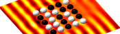
Why not take a break and have a slice of the following figure before reading on.
)
An electromagnetic wave scattering off a perfectly conducting metal cake. This solution was found using a Calderón preconditioned boundary element method.
Previous post in series

This is the second post in a series of posts about my PhD thesis.
Next post in series

(Click on one of these icons to react to this blog post)
You might also enjoy...

Comments
Comments in green were written by me. Comments in blue were not written by me.
Add a Comment
2020-01-31
This is the first post in a series of posts about my PhD thesis.
Yesterday, I handed in the final version of my PhD thesis. This is the first in a series of blog posts in which I will attempt to explain what my thesis says with minimal
mathematical terminology and notation.
The aim of these posts is to give a more general audience some idea of what my research is about. If you are looking to build on my work, I recommend that you read
my thesis, or my papers based on parts of it for the full mathematical detail. You may find these posts helpful
with developing a more intuitive understanding of some of the results in these.
In this post, we start at the beginning and look at what is contained in chapter 1 of my thesis.
Introduction
In general, my work looks at using discretisation to approximately solve partial differential equations (PDEs). We primarily focus on three PDEs:
| Laplace's equation | \(-\Delta u=0\) |
If \(u\) represents the temperature in a region,
the region contains no heat sources, and the heat distribution in the region is not changing, then \(u\) a solution of Laplace's equation.
Because of this application, Laplace's equation is sometimes called the steady-state heat equation.
| The Helmholtz equation | \(-\Delta u-k^2u=0\) |
The Helmholtz equation models acoustic waves travelling through a medium.
The unknown \(u\) represents the amplitude of the wave at each point.
The equation features the wavenumber \(k\), which gives the number of waves per unit distance.
| Maxwell's equations | \(\nabla\times\nabla\times e-k^2e=0\) |
Maxwell's equations describe the behaviour of electromagnetic waves. The unknown \(e\) in Maxwell's equatons is an unknown vector, whereas the unknown \(u\) in Laplace and Helmholtz is a scalar.
This adds some difficulty when working with Maxwell's equations.
Discretisation
In many situations, no method for finding the exact solution to these equations is known. It is therefore very important to be able to get accurate approximations of the
solutions of these equations. My PhD thesis focusses on how these can be approximately solved using discretisation.
Each of the PDEs that we want to solve describes a function that has a value at every point in a 3D space: there are an (uncountably) infinite number of points, so these
equations effectively have an infinite number of unknown values that we want to know. The aim of discretisation is to reduce the number of unknowns to a finite number in such a way that
solving the finite problem gives a good approximation of the true solution. The finite problem can then be solved using your favourite matrix method.
For example, we could split a 2D shape into lots of small triangles, or split a 3D shape into lots of small tetrahedra. We could then try to approximate our solution with a constant inside
each triangle or tetrahedron. Or we could approximate by taking a value at each vertex of the triangles or tetrahedra, and a linear function inside shape. Or we could use quadratic functions or higher
polynomials to approximate the solution. This is the approach taken by a method called the finite element method.
My thesis, however, focusses on the boundary element method, a method that is closely related to the finite element method. Imagine that we want to solve a PDE problem inside a sphere.
For some PDEs (such as the three above), it is possible to represent the solution in terms of some functions on the surface of the sphere. We can then approximate the solution to the problem
by approximating these functions on the surface: we then only have to discretise the surface and not the whole of the inside of the sphere. This method will also work for other 3D shapes, and isn't
limited to spheres.
One big advantage of this method is that it can also be used if we want to solve a problem in the (infinte) region outside an object, as even if the region is infinite, the surface of the object
will be finite. The finite element method has difficulties here, as splitting the infinite region in tetrahedra would require an infinite number of tetrahedra, which destroys the point of discretisation
(although this kind of problem can be solved using finite elements if you split into tetrahedra far enough outwards, then use some tricks where your tetrahedron stop). The finite element method, on the
other hand, works for a much wider range of PDEs, so in many situations it would be the only of these two methods that can be used.
We focus on the boundary element method as when it can be used, it can be a very powerful method.
Sobolev spaces
Much of the first chapter of my thesis looks at the definitions of Sobolev function spaces: these spaces describe the types of functions that we will look for to solve our PDEs.
It is important to frame the problems using Sobolev spaces, as properties of these spaces are used heavily when proving results about our approximations.
The definitions of these spaces are too technical to include here, but the spaces can be thought of as a way to require certain things of the solutions to our problems.
We start be demanding that the function be square integrable: they can be squared the integrated to give a finite answer. Other spaces are then defined by demanding that a
function can be differentiated to give a square integrable derivative; or it can be differentiated twice or more times.
Boundary element method
We now look at how the boundary element method works in more detail. The "boundary" in the name refers to the surface of the object or region that we are solving problems in.
In order to be able to use the boundary element method, we need to know the Green's function of the PDE in question.
(This is what limits the number of problems that the boundary element method can be used to solve.)
The Green's function is the solution as every point in 3D (or 2D if you prefer) except for one point, where it has an infinite value, but a very special type of infinite value.
The Green's function gives the field due to a unit point source at the chosen point.
If a region contains no sources, then the solution inside that region can be represented by adding up point sources at every point on the boundary (or in other words, integrating the Green's function
times a weighting function, as the limit of adding up these at lots of points is an integral). The solution could instead be represented by doing the same thing with the derivative of the Green's function.
We define two potential operators—the single layer potential \(\mathcal{V}\) and the double layer potential \(\mathcal{K}\)—to be the two operators representing the two boundary integrals:
these operators can be applied to weight functions on the boundary to give solutions to the PDE in the region. Using these operators, we write a representation formula that tells us how
to compute the solution inside the region once we know the weight functions on the boundary.
By looking at the values of these potential operators on the surface, and derivative of these values, (and integrating these over the boundary) we can define four boundary operators:
the single layer operator \(\mathsf{V}\),
the double layer operator \(\mathsf{K}\),
the adjoint double layer operator \(\mathsf{K}'\),
the hypersingular operator \(\mathsf{W}\).
We use these operators to write the boundary integral equation that we derive from the representation formula. It is this boundary integral equation that we will apply discretisation
to to find an approximation of the weight functions; we can then use the representation formula to find the solution to the PDE.
The Calderón projector
Using the four boundary operators, we can define the Calderón projector, \(\mathsf{C}\):
$$\mathsf{C}=\begin{bmatrix}
\tfrac12-\mathsf{K}&\mathsf{V}\\
\mathsf{W}&\tfrac12+\mathsf{K}'
\end{bmatrix}$$
This is the Calderón projector for problems in a finite interior region. For exterior problems, the exterior Cadleró is used. This is given by
$$\mathsf{C}=\begin{bmatrix}
\tfrac12+\mathsf{K}&-\mathsf{V}\\
-\mathsf{W}&\tfrac12-\mathsf{K}'
\end{bmatrix}.$$
We treat the Calderón operator like a matrix, even though its entries are operators not numbers. The Calderón projector has some very useful properties that
are commonly used when using the boundary element method. These include:
- \(\mathsf{C}^2=\mathsf{C}\).
- If we apply \(\mathsf{C}\) to a solution of the PDE, the Calderón projector does nothing to the input.
- If we apply \(\mathsf{C}\) to any functions, the result will be a solution of the PDE.
These properties conclude chapter 1 of my thesis. Why not take a break and fill the following diagram with hot liquid before reading on.
)
The results of applying the Calderón projector to two functions. By the properties above, these are (the boundary traces of) a solution of the PDE.
This is the first post in a series of posts about my PhD thesis.
Next post in series
(Click on one of these icons to react to this blog post)
You might also enjoy...
Comments
Comments in green were written by me. Comments in blue were not written by me.
Add a Comment
2020-01-24
This is the second post in a series of posts about matrix methods.
We want to solve \(\mathbf{A}\mathbf{x}=\mathbf{b}\), where \(\mathbf{A}\) is a (known) matrix, \(\mathbf{b}\) is a (known) vector, and \(\mathbf{x}\) is an unknown vector.
This matrix system can be thought of as a way of representing simultaneous equations. For example, the following matrix problem and system of simultaneous equations are equivalent.
\begin{align*}
\begin{pmatrix}2&1\\3&1\end{pmatrix}\mathbf{x}&=\begin{pmatrix}3\\4\end{pmatrix}
&&\quad&&
\begin{array}{r}
2x+2y=3&\\
3x+2y=4&
\end{array}
\end{align*}
The simultaneous equations here would usually be solved by adding or subtracting the equations together. In this example, subtracting the first equation from the second gives \(x=1\).
From there, it is not hard to find that \(y=\frac12\).
One approach to solving \(\mathbf{A}\mathbf{x}=\mathbf{b}\) is to find the inverse matrix \(\mathbf{A}^{-1}\), and use \(\mathbf{x}=\mathbf{A}^{-1}\mathbf{b}\). In this post, we use Gaussian elimination—a method
that closely resembles the simultaneous equation method—to find \(\mathbf{A}^{-1}\).
Gaussian elimination
As an example, we will use Gaussian elimination to find the inverse of the matrix
$$\begin{pmatrix}
1&-2&4\\
-2&3&-2\\
-2&2&2
\end{pmatrix}.$$
First, write the matrix with an identity matrix next to it.
$$\left(\begin{array}{ccc|ccc}
1&-2&4&1&0&0\\
-2&3&-2&0&1&0\\
-2&2&2&0&0&1
\end{array}\right)$$
Our aim is then to use row operations to change the matrix on the left of the vertical line into the identity matrix, as
the matrix on the right will then be the inverse. We are allowed to use two row operations: we can multiply a row by a scalar; or we can add a multiple of a row to another row.
These operations closely resemble the steps used to solve simultaneous equations.
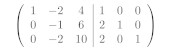
We will get the matrix to the left of the vertical line to be the identity in a systematic manner: our first aim is to get the first column to read 1, 0, 0.
We already have the 1; to get the 0s, add 2 times the first row to both the second and third rows.
$$\left(\begin{array}{ccc|ccc}
1&-2&4&1&0&0\\
0&-1&6&2&1&0\\
0&-2&10&2&0&1
\end{array}\right)$$
Our next aim is to get the second column to read 0, 1, 0. To get the 1, we multiply the second row by -1.
$$\left(\begin{array}{ccc|ccc}
1&-2&4&1&0&0\\
0&1&-6&-2&-1&0\\
0&-2&10&2&0&1
\end{array}\right)$$
To get the 0s, we add 2 times the second row to both the first and third rows.
$$\left(\begin{array}{ccc|ccc}
1&0&-8&-3&-2&0\\
0&1&-6&-2&-1&0\\
0&0&-2&-2&-2&1
\end{array}\right)$$
Our final aim is to get the third column to read 0, 0, 1. To get the 1, we multiply the third row by -½.
$$\left(\begin{array}{ccc|ccc}
1&0&-8&-3&-2&0\\
0&1&-6&-2&-1&0\\
0&0&1&1&1&-\tfrac{1}{2}
\end{array}\right)$$
To get the 0s, we add 8 and 6 times the third row to the first and second rows (respectively).
$$\left(\begin{array}{ccc|ccc}
1&0&0&5&6&-4\\
0&1&0&4&5&-3\\
0&0&1&1&1&-\tfrac{1}{2}
\end{array}\right)$$
We have the identity on the left of the vertical bar, so we can conclude that
$$\begin{pmatrix}
1&-2&4\\
-2&3&-2\\
-2&2&2
\end{pmatrix}^{-1}
=
\begin{pmatrix}
5&6&-4\\
4&5&-3\\
1&1&-\tfrac{1}{2}
\end{pmatrix}.$$
How many operations
This method can be used on matrices of any size. We can imagine doing this with an \(n\times n\) matrix and look at how many operations
the method will require, as this will give us an idea of how long this method would take for very large matrices.
Here, we count each use of \(+\), \(-\), \(\times\) and \(\div\) as a (floating point) operation (often called a flop).
Let's think about what needs to be done to get the \(i\)th column of the matrix equal to 0, ..., 0, 1, 0, ..., 0.
First, we need to divide everything in the \(i\)th row by the value in the \(i\)th row and \(i\)th column. The first \(i-1\) entries in the column will already be 0s though, so there is no need to divide
these. This leaves \(n-(i-1)\) entries that need to be divided, so this step takes \(n-(i-1)\), or \(n+1-i\) operations.
Next, for each other row (let's call this the \(j\)th row), we add or subtract a multiple of the \(i\)th row from the \(j\)th row. (Again the first \(i-1\) entries can be ignored as they are 0.)
Multiplying the \(i\)th row takes \(n+1-i\) operations, then adding/subtracting takes another \(n+1-i\) operations.
This needs to be done for \(n-1\) rows, so takes a total of \(2(n-1)(n+1-i)\) operations.
After these two steps, we have finished with the \(i\)th column, in a total of \((2n-1)(n+1-i)\) operations.
We have to do this for each \(i\) from 1 to \(n\), so the total number of operations to complete Gaussian elimination is
$$
(2n-1)(n+1-1)
+
(2n-1)(n+1-2)
+...+
(2n-1)(n+1-n)
$$
This simplifies to
$$\tfrac12n(2n-1)(n+1)$$
or
$$n^3+\tfrac12n^2-\tfrac12n.$$
The highest power of \(n\) is \(n^3\), so we say that this algorithm is an order \(n^3\) algorithm, often written \(\mathcal{O}(n^3)\).
We focus on the highest power of \(n\) as if \(n\) is very large, \(n^3\) will be by far the largest number in the expression, so gives us an idea of how fast/slow this algorithm will be for large
matrices.
\(n^3\) is not a bad start—it's far better than \(n^4\), \(n^5\), or \(2^n\)—but there are methods out there that will take less than \(n^3\) operations.
We'll see some of these later in this series.
Previous post in series
This is the second post in a series of posts about matrix methods.
Next post in series
(Click on one of these icons to react to this blog post)
You might also enjoy...
Comments
Comments in green were written by me. Comments in blue were not written by me.
Add a Comment
2020-01-23
This is the first post in a series of posts about matrix methods.
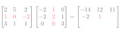
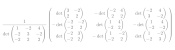
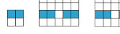
When you first learn about matrices, you learn that in order to multiply two matrices, you use this strange-looking method involving the rows of the left matrix and the columns of this right.
)
It doesn't immediately seem clear why this should be the way to multiply matrices. In this blog post, we look at why this is the definition of matrix multiplication.
Simultaneous equations
Matrices can be thought of as representing a system of simultaneous equations. For example, solving the matrix problem
$$
\begin{bmatrix}2&5&2\\1&0&-2\\3&1&1\end{bmatrix}
\begin{pmatrix}x\\y\\z\end{pmatrix}
=
\begin{pmatrix}14\\-16\\-4\end{pmatrix}
$$
is equivalent to solving the following simultaneous equations.
\begin{align*}
2x+5y+2z&=14\\
1x+0y-2z&=-16\\
3x+1y+1z&=-4
\end{align*}
Two matrices
Now, let \(\mathbf{A}\) and \(\mathbf{C}\) be two 3×3 matrices, let \(\mathbf{b}\) by a vector with three elements, and let \(\mathbf{x}=(x,y,z)\).
We consider the equation
$$\mathbf{A}\mathbf{C}\mathbf{x}=\mathbf{b}.$$
In order to understand what this equation means, we let \(\mathbf{y}=\mathbf{C}\mathbf{x}\) and think about solving the two simuntaneous matrix equations,
\begin{align*}
\mathbf{A}\mathbf{y}&=\mathbf{b}\\
\mathbf{C}\mathbf{x}&=\mathbf{y}.
\end{align*}
We can write the entries of \(\mathbf{A}\), \(\mathbf{C}\), \(\mathbf{x}\), \(\mathbf{y}\) and \(\mathbf{b}\) as
\begin{align*}
\mathbf{A}&=\begin{bmatrix}
a_{11}&a_{12}&a_{13}\\
a_{21}&a_{22}&a_{23}\\
a_{31}&a_{32}&a_{23}
\end{bmatrix}
&
\mathbf{C}&=\begin{bmatrix}
c_{11}&c_{12}&c_{13}\\
c_{21}&c_{22}&c_{23}\\
c_{31}&c_{32}&c_{23}
\end{bmatrix}
\end{align*}
\begin{align*}
\mathbf{x}&=\begin{pmatrix}x_1\\x_2\\x_3\end{pmatrix}
&
\mathbf{y}&=\begin{pmatrix}y_1\\y_2\\y_3\end{pmatrix}
&
\mathbf{b}&=\begin{pmatrix}b_1\\b_2\\b_3\end{pmatrix}
\end{align*}
We can then write out the simultaneous equations that \(\mathbf{A}\mathbf{y}=\mathbf{b}\) and \(\mathbf{C}\mathbf{x}=\mathbf{y}\) represent:
\begin{align}
a_{11}y_1+a_{12}y_2+a_{13}y_3&=b_1&
c_{11}x_1+c_{12}x_2+c_{13}x_3&=y_1\\
a_{21}y_1+a_{22}y_2+a_{23}y_3&=b_2&
c_{21}x_1+c_{22}x_2+c_{23}x_3&=y_2\\
a_{31}y_1+a_{32}y_2+a_{33}y_3&=b_3&
c_{31}x_1+c_{32}x_2+c_{33}x_3&=y_3\\
\end{align}
Substituting the equations on the right into those on the left gives:
\begin{align}
a_{11}(c_{11}x_1+c_{12}x_2+c_{13}x_3)+a_{12}(c_{21}x_1+c_{22}x_2+c_{23}x_3)+a_{13}(c_{31}x_1+c_{32}x_2+c_{33}x_3)&=b_1\\
a_{21}(c_{11}x_1+c_{12}x_2+c_{13}x_3)+a_{22}(c_{21}x_1+c_{22}x_2+c_{23}x_3)+a_{23}(c_{31}x_1+c_{32}x_2+c_{33}x_3)&=b_2\\
a_{31}(c_{11}x_1+c_{12}x_2+c_{13}x_3)+a_{32}(c_{21}x_1+c_{22}x_2+c_{23}x_3)+a_{33}(c_{31}x_1+c_{32}x_2+c_{33}x_3)&=b_3\\
\end{align}
Gathering the terms containing \(x_1\), \(x_2\) and \(x_3\) leads to:
\begin{align}
(a_{11}c_{11}+a_{12}c_{21}+a_{13}c_{31})x_1
+(a_{11}c_{12}+a_{12}c_{22}+a_{13}c_{32})x_2
+(a_{11}c_{13}+a_{12}c_{23}+a_{13}c_{33})x_3&=b_1\\
(a_{21}c_{11}+a_{22}c_{21}+a_{23}c_{31})x_1
+(a_{21}c_{12}+a_{22}c_{22}+a_{23}c_{32})x_2
+(a_{21}c_{13}+a_{22}c_{23}+a_{23}c_{33})x_3&=b_2\\
(a_{31}c_{11}+a_{32}c_{21}+a_{33}c_{31})x_1
+(a_{31}c_{12}+a_{32}c_{22}+a_{33}c_{32})x_2
+(a_{31}c_{13}+a_{32}c_{23}+a_{33}c_{33})x_3&=b_3
\end{align}
We can write this as a matrix:
$$
\begin{bmatrix}
a_{11}c_{11}+a_{12}c_{21}+a_{13}c_{31}&
a_{11}c_{12}+a_{12}c_{22}+a_{13}c_{32}&
a_{11}c_{13}+a_{12}c_{23}+a_{13}c_{33}\\
a_{21}c_{11}+a_{22}c_{21}+a_{23}c_{31}&
a_{21}c_{12}+a_{22}c_{22}+a_{23}c_{32}&
a_{21}c_{13}+a_{22}c_{23}+a_{23}c_{33}\\
a_{31}c_{11}+a_{32}c_{21}+a_{33}c_{31}&
a_{31}c_{12}+a_{32}c_{22}+a_{33}c_{32}&
a_{31}c_{13}+a_{32}c_{23}+a_{33}c_{33}
\end{bmatrix}
\mathbf{x}=\mathbf{b}
$$
This equation is equivalent to \(\mathbf{A}\mathbf{C}\mathbf{x}=\mathbf{b}\), so the matrix above is equal to \(\mathbf{A}\mathbf{C}\). But this matrix is what you get if follow the
row-and-column matrix multiplication method, and so we can see why this definition makes sense.
This is the first post in a series of posts about matrix methods.
Next post in series
(Click on one of these icons to react to this blog post)
You might also enjoy...
Comments
Comments in green were written by me. Comments in blue were not written by me.
Add a Comment
2020-01-02
It's 2020, and the Advent calendar has disappeared, so it's time to reveal the answers and annouce the winners.
But first, some good news: with your help, Santa and his two reindeer were found and Christmas was saved!
Now that the competition is over, the questions and all the answers can be found here.
Before announcing the winners, I'm going to go through some of my favourite puzzles from the calendar, reveal the solution and a couple of notes and Easter eggs.
Highlights
My first highlight is this puzzle from 10 December that seems difficult to get started on, but plotting the two quadratics reveals a very useful piece of information that can be used.
10 December
For all values of \(x\), the function \(f(x)=ax+b\) satisfies
$$8x-8-x^2\leqslant f(x)\leqslant x^2.$$
What is \(f(65)\)?
Edit: The left-hand quadratic originally said \(8-8x-x^2\). This was a typo and has now been corrected.
)
My next highlight is the puzzle from 12 December, which was election day in the UK. Although the puzzle isn't that difficult or interesting to calculate, the answer is surprising enough
to make this one of my favourites.
12 December
For a general election, the Advent isles are split into 650 constituencies. In each constituency, exactly 99 people vote: everyone votes for one of the two main parties: the Rum party or the
Land party. The party that receives the most votes in each constituency gets an MAP (Member of Advent Parliament) elected to parliament to represent that constituency.
In this year's election, exactly half of the 64350 total voters voted for the Rum party. What is the largest number of MAPs that the Rum party could have?
My next highlight is the puzzle from 13 December. If you enjoyed this one, then you can find a puzzle based on a similar idea on the puzzles
pages of issue 10 of Chalkdust.
13 December
Each clue in this crossnumber (except 5A) gives a property of that answer that is true of no other answer. For example: 7A is a multiple of 13; but 1A, 3A, 5A, 1D, 2D, 4D, and 6D are all not multiples of 13.
No number starts with 0.
|
| ||||||||||||||||||||||||||||||||||||||||||||||
My final highlight is the puzzle from 16 December. I always include a few of these, as they can be designed to give any answer so are useful for making the final logic puzzle work.
But I was particularly happy with this one.
16 December
Arrange the digits 1-9 in a 3×3 square so that:
the median number in the first row is 6;
the median number in the second row is 3;
the mean of the numbers in the third row is 4;
the mean of the numbers in the second column is 7;
the range of the numbers in the third column is 2,
The 3-digit number in the first column is today's number.
| median 6 | |||
| median 3 | |||
| mean 4 | |||
| today's number | mean 7 | range 2 |
Notes and Easter eggs
A few of you may have noticed the relevance of the colours assigned to each island:
Rum (Red Rum),
Land (Greenland),
Moon (Blue Moon), and
County (Orange County).
Once you've entered 24 answers, the calendar checks these and tells you how many are correct. I logged the answers that were sent
for checking and have looked at these to see which puzzles were the most and least commonly incorrect. The bar chart below shows the total number
of incorrect attempts at each question.
| 1 | 2 | 3 | 4 | 5 | 6 | 7 | 8 | 9 | 10 | 11 | 12 | 13 | 14 | 15 | 16 | 17 | 18 | 19 | 20 | 21 | 22 | 23 | 24 |
| Day | |||||||||||||||||||||||
You can see that the most difficult puzzles were those on
4 and
15 December;
and the easiest puzzles were on
3,
11,
17, and
24 December.
This year, the final logic puzzle revealed the positions of Santa, Rudolph and Blitzen, then you had to find them on this map.
The map has 6 levels, with 81 positions on each level, so the total size of the map is \(81^6=282\,429\,536\,481\) squares.
This is a lot; one Advent solver even wondered how large a cross stitch of the whole thing would be.
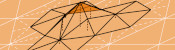
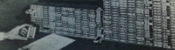
I obviously didn't draw 282 billion tiles: the whole map was generated using the following tiles, which were reused across the map.
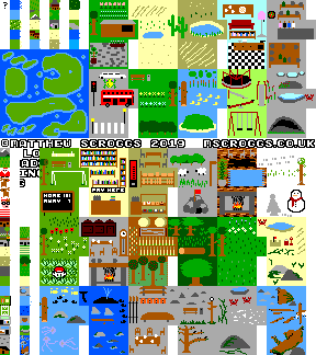
The map tiles.
I also snuck a small Easter egg into the map. Below the Advent calendar, this example was shown:
)
The ASC coordinates of this pair of flowers are 12.52.12.13.84.55 (click to enlarge).
If you actually visited this position on the map, you found Wally.
)
Wally.
At least one Advent solver appears to have found Wally, as they left this cryptic comment under the name Dr Matrix
(an excellent Martin Gardner reference).
The solution
The solutions to all the individual puzzles can be found here.
Using the daily clues, it was possible to work out that
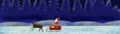
Santa was at 36.11.19.79.79.43, Blitzen was at 23.12.23.11.23.11, and Rudolph was at 16.64.16.16.16.64.
)
Santa (left), Blitzen (centre) and Rudolph (right).
The winners
And finally (and maybe most importantly), on to the winners: 126 people found Santa and both reindeer and entered the competition. Their (very) approximate locations are shown on this map:
)
From the correct answers, the following 10 winners were selected:
| 1 | Valentin Valciu |
| 2 | Tom Anderson |
| 3 | Alex Bolton |
| 4 | Kevin Fray |
| 5 | Jack Kiuttu |
| 6 | Ben Baker |
| 7 | Joe Gage |
| 8 | Michael Thomas |
| 9 | Martin Holtham |
| 10 | Beth Jensen |
Congratulations! Your prizes will be on their way shortly.
The prizes this year include 2019 Advent calendar T-shirts. If you didn't win one, but would like one of these, you can buy one at mscroggs.co.uk/tshirt until 7 January
(when I will be sending them for printing).
)
The design on the T-shirt.
Additionally, well done to
Adam Abrams, Adam NH, Adam Vellender, Alan Buck, Alex Ayres, Alex Burlton, Alexander Ignatenkov, Andrew Ennaco, Andrew Tindall, Artie Smith, Ashley Jarvis, Austin Antoniou, Becky Russell,
Ben Jones, Ben Reiniger, Brennan Dolson, Brian Carnes, Carl Westerlund, Carmen Guenther, Clare Wallace, Colin Beveridge, Connie, Corbin Groothuis, Cory Peters, Dan Colestock, Dan DiMillo,
Dan Whitman, David, David Ault, David Fox, Diane Keimel, Duncan Ramage, Emilie Heidenreich, Emily Troyer, Eric, Eric Kolbusz, Erik Eklund, Evan Louis Robinson, Frances Haigh, Franklin Ta,
Fred Verheul, Félix Breton, Gabriella Pinter, Gautam Webb, Gert-Jan de Vries, Hart Andrin, Heerpal Sahota, Herschel Pecker, Jacob Juillerat, Jan, Jean-Noël Monette, Jen Shackley,
Jeremiah Southwick, Jessica Marsh, Johan Asplund, John Warwicker, Jon Foster, Jon Palin, Jonathan Chaffer, Jonathan Winfield, Jose, Kai, Karen Climis, Karen Kendel, Katja Labermeyer, Laura,
Lewis Dyer, Louis de Mendonca, M Oostrom, Magnus Eklund, Mahmood Hikmet, Marian Clegg, Mark Stambaugh, Martin Harris, Martine Vijn Nome, Matt Hutton, Matthew Askins, Matthew Schulz,
Maximilian Pfister, Melissa Lucas, Mels, Michael DeLyser, Michael Gustin, Michael Horst, Michael Prescott, Mihai Zsisku, Mike, Mikko, Moreno Gennari, Nadine Chaurand, Naomi Bowler, Nathan C,
Pat Ashforth, Paul Livesey, Pranshu Gaba, Raymond Arndorfer, Riccardo Lani, Rosie Paterson, Rupinder Matharu, Russ Collins, S A Paget, SShaikh, Sam Butler, Sam Hartburn, Scott, Seth Cohen,
Shivanshi Adlakha, Simon Schneider, Stephen Cappella, Stephen Dainty, Steve Blay, Thomas Tu, Tom Anderson, Tony Mann, Yasha, and Yuliya Nesterova,
who all also submitted the correct answer but were too unlucky to win prizes this time.
See you all next December, when the Advent calendar will return.
(Click on one of these icons to react to this blog post)
You might also enjoy...


Comments
Comments in green were written by me. Comments in blue were not written by me.
It's interesting that the three puzzles with the most incorrect attempts can all be looked up on OEIS.
Day 15 - https://oeis.org/A001055 - "number of ways of factoring n with all factors greater than 1"
Day 4 - https://oeis.org/A001045 - "number of ways to tile a 2 × (n-1) rectangle with 1 × 2 dominoes and 2 × 2 squares"
Day 2 - https://oeis.org/A002623 - "number of nondegenerate triangles that can be made from rods of length 1,2,3,4,...,n" ×1
×1
Day 15 - https://oeis.org/A001055 - "number of ways of factoring n with all factors greater than 1"
Day 4 - https://oeis.org/A001045 - "number of ways to tile a 2 × (n-1) rectangle with 1 × 2 dominoes and 2 × 2 squares"
Day 2 - https://oeis.org/A002623 - "number of nondegenerate triangles that can be made from rods of length 1,2,3,4,...,n"
Adam Abrams
Never mind, I found them, they were your example ASC. Very clever! ×1
Michael T
Where did the coordinates for Wally come from? Are they meaningful, or are they just some random coordinates thrown together?
Michael T
Add a Comment