
Blog
2015-10-21
This post also appeared on the Chalkdust Magazine blog.
If you're like me, then you will be disappointed that all of the home nations have been knocked out of the Rugby World Cup. If you're really like me, doing some maths related to rugby will cheer you up...
The scoring system in rugby awards points in packets of 3, 5 and 7. This leads a number of interesting questions that you can find in my guest puzzle on Alex Bellos's Guardian blog. In this blog post, we will focus on another area of rugby: conversion kicking.
Conversion kicks
When a try is scored by putting the ball down behind the line, the scoring team gets to take a conversion kick. This kick must be taken in line with where the try was scored but it is up to the kicker how far away the kick should be taken. But how far back should the ball be taken to make the kick easiest?
)
Too close (red) and too far away (blue) will give small angles to aim at. Somewhere in the middle is needed (green).
One way to answer this question is to look to maximise the angle between the posts which the kicker will have to aim at: if the kick is taken too close to or too far from the goal line there will be a very thin angle to aim at. Somewhere between these extremes there will be a maximum angle to aim at.
When looking to maximise this angle, we can use one of the 'circle theorems' which have tormented many generations of GCSE maths students: 'angles subtended by the same arc at the circumference are equal'. This means that if a circle is drawn going through both posts, then the angle made at any point on this circle will be the same.
)
The angles made by the red and blue lines are equal because 'angles subtended by the same arc at the circumference are equal'.
A larger circle drawn through the posts will give a smaller angle. If a vertical line is drawn which just touches the right of the circle, then the point at which it touches the circle will be the best place on this line to take a kick. This is because any other point on the line will be on a larger circle and so make a smaller angle.
Using this method for circles of different sizes leads to the following diagram, which shows where the kick should be taken for every position a try could be scored:
)
The best place to take a kick?
This, however, is not the best place to take the kick.
Taking account of height
When a try is scored near the posts, the above method recommends a position from where the ball must be kicked at an impossibly steep angle to go over. To deal with this problem, we are going to have to look at the situation from the side.
When kicked, the ball will travel along a parabola (ignoring air resistance and wind as their effects will be small[citation needed]). Given a distance from the posts, there will be two angles which the ball can be kicked at and just make it over the bar. Kicking at any angle between these two will lead to a successful conversion. Again, we have an angle which we would like to maximise.
)
The highest (blue) and lowest (red) the ball can be kicked while still going over the bar.
However, the position where this angle is maximised is very unlikely to also maximise the angle we looked at earlier. To find the best place to kick from, we need to find a compromise point where both angles are quite big.
To do this, imagine that the kicker is standing inside a large sphere. For each point on the sphere, kicking the ball at the point will either lead to it going over or missing. We can draw a shape on the sphere so that aiming inside the shape will lead to scoring. Our sensible kicker will aim at the centre of this shape.
But our kicker will not be able to aim perfectly: there will be some random variation. We can predict that this variation will follow a Kent distribution, which is like a normal distribution but on the surface of a sphere. We can use this distribution to calculate the probability that our kicker will score. We would like to maximise this probability.
The Kent distribution can be adjusted to reflect the accuracy of the kicker. Below are the optimal kicking positions for an inaccurate, an average and a very accurate kicker.
)
)
)
The best place to take a kick for a bad kicker (top), an average kicker (middle) and a good kicker (bottom). All the kickers kick the ball at 30m/s.
As you might expect, the less accurate kicker should stand slightly further forwards to make it easier to aim. Perhaps surprisingly, the good kicker should stand further back when between the posts than when in line with the posts.
The model used to create these results could be further refined. Random variation in the speed of the kick could be introduced. Or the kick could be made to have more variation horizontally than vertically: there are parameters in the Kent distribution which allow this to be easily adjusted. In fact, data from players could be used to determine the best position for each player to kick from.
In addition to analysing conversions, this method could be used to determine the probability of scoring 3 points from any point on the pitch. This could be used in conjunction with the probability of scoring a try from a line-out to decide whether kicking a penalty for the posts or into touch is likely to lead to the most points.
Although estimating the probability of scoring from a line-out is a difficult task. Perhaps this will give you something to think about during the remaining matches of the tournament.
(Click on one of these icons to react to this blog post)
You might also enjoy...

Comments
Comments in green were written by me. Comments in blue were not written by me.
Add a Comment
2015-10-08
This post also appeared on the Chalkdust Magazine blog. You can read the excellent second issue of Chalkdust here, including the £100 prize crossnumber which I set.
From today, the National Lottery's Lotto draw has 59 balls instead of 49. You may be thinking that this means there is now much less chance of winning. You would be right, except the prizes are also changing.
Camelot, who run the lottery, are saying that you are now "more likely to win a prize" and "more likely to become a millionaire". But what do these changes actually mean?
The changes
Until yesterday, Lotto had 49 balls. From today, there are 59 balls. Each ticket still has six numbers on it and six numbers, plus a bonus ball, are still chosen by the lottery machine. The old prizes were as follows:
| Requirement | Estimated Prize |
| Match all 6 normal balls | £2,000,000 |
| Match 5 normal balls and the bonus ball | £50,000 |
| Match 5 normal balls | £1,000 |
| Match 4 normal balls | £100 |
| Match 3 normal balls | £25 |
| 50 randomly picked tickets | £20,000 |
The prizes have changed to:
| Requirement | Estimated Prize |
| Match all 6 normal balls | £2,000,000 |
| Match 5 normal balls and the bonus ball | £50,000 |
| Match 5 normal balls | £1,000 |
| Match 4 normal balls | £100 |
| Match 3 normal balls | £25 |
| Match 2 normal balls | Free lucky dip entry in next Lotto draw |
| One randomly picked ticket | £1,000,000 |
| 20 other randomly picked tickets | £20,000 |
Probability of Winning a Prize
The probability of winning each of these prizes can be calculated. For example, the probability of matching all 6 balls in the new lotto is $$\mathbb{P}(\mathrm{matching\ ball\ 1})\times \mathbb{P}(\mathrm{matching\ ball\ 2})\times...\times\mathbb{P}(\mathrm{matching\ ball\ 6})$$ $$=\frac{6}{59}\times\frac{5}{58}\times\frac{4}{57}\times\frac{3}{56}\times\frac{2}{55}\times\frac{1}{54}$$ $$=\frac{1}{45057474},$$ and the probability of matching 4 balls in the new lotto is $$(\mathrm{number\ of\ different\ ways\ of\ picking\ four\ balls\ out\ of\ six})\times\mathbb{P}(\mathrm{matching\ ball\ 1})\times\\...\times\mathbb{P}(\mathrm{matching\ ball\ 4})\times\mathbb{P}(\mathrm{not\ matching\ ball\ 5})\times\mathbb{P}(\mathrm{not\ matching\ ball\ 6})$$ $$=15\times\frac{6}{59}\times\frac{5}{58}\times\frac{4}{57}\times\frac{3}{56}\times\frac{53}{55}\times\frac{52}{54}$$ $$=\frac{3445}{7509579}.$$ In the second calculation, it is important to include the probabilities of not matching the other balls to prevent double counting the cases when more than 4 balls are matched.
Calculating a probability for every prize and then adding them up gives the probability of winning a prize. In the old draw, the probability of winning a prize was \(0.0186\). In the new draw, it is \(0.1083\). So Camelot are correct in claiming that you are now more likely to win a prize.
But not all prizes are equal: these probabilities do not take into account the values of the prizes. To analyse the actual winnings, we're going to have to look at the expected amount of money you will win. But first, let's look at Camelot's other claim: that under the new rules you are more likely to become a millionaire.
Probability of winning £1,000,000
In the old draw, the only way to win a million pounds was to match all six balls. The probability of this happening was \(0.00000007151\) or \(7.151\times 10^{-8}\).
In the new lottery, a million pounds can be won either by matching all six balls or by winning the millionaire raffle. This will lead to different probabilities of winning on Wednesdays and Saturdays due to different numbers of people buying tickets. Based on expected sales of 16.5 million tickets on Saturdays and 8.5 million tickets on Wednesdays, the chances of becoming a millionaire on a Wednesday or Saturday are \(0.0000001398\) (\(1.398\times 10^{-7}\)) and \(0.00000008280\) (\(8.280\times 10^{-8}\)) respectively.
These are both higher than the probability of winning a million in the old draw, so again Camelot are correct: you are now more likely to become a millionaire...
But the new chances of becoming a millionaire are actually even higher. The probabilities given above are the chances of winning a million in a given draw. But if two balls are matched, you win a lucky dip: you could win a million in the next draw without buying another ticket. We should include this in the probability calculated above, as you are still becoming a millionaire due to the original ticket you bought.
In order to count this, let \(A_W\) and \(A_S\) be the probabilities of winning a million in a given draw (as given above) on a Wednesday or a Saturday, let \(B_W\) and \(B_S\) be the probabilities of winning a million in this draw or due to future lucky dip tickets on a Wednesday or a Saturday (the values we want to find) and let \(p\) be the probability of matching two balls. We can write $$B_W=A_W+pB_S$$ and $$B_S=A_S+pB_W$$ since the probability of winning a million is the probability of winning in this draw (\(A\)) plus the probability of winning a lucky dip ticket and winning in the next draw (\(pB\)). Substituting and rearranging, we get $$B_W=\frac{A_W+pA_S}{1-p^2}$$ and $$B_W=\frac{A_S+pA_W}{1-p^2}.$$
Using this (and the values of \(A_S\) and \(A_W\) calculated earlier) gives us probabilities of \(0.0000001493\) (\(1.493\times 10^{-7}\)) and \(0.00000009736\) (\(9.736\times 10^{-8}\)) of becoming a millionaire on a Wednesday and a Saturday respectively. These are both significantly higher than the probability of becoming a millionaire in the old draw (\(7.151\times 10^{-8}\)).
Camelot's two claims—that you are more likely to win a prize and you are more likely to become a millionaire—are both correct. It sounds like the new lottery is a great deal, but so far we have not taken into account the size of the prizes you will win and have only shown that a very rare event will become slightly less rare. Probably the best way to measure how good a lottery is is by working out the amount of money you should expect to win, so let's now look at that.
Expected prize money
To find the expected prize money, we must multiply the value of each prize by the probability of winning that prize and then add them up, or, in other words,
$$\sum_\mathrm{prizes}\mathrm{value\ of\ prize}\times\mathbb{P}(\mathrm{winning\ prize}).$$
Once this has been calculated, the chance of winning due to a free lucky dip entry must be taken into account as above.
In the old draw, after buying a ticket for £2, you could expect to win 78p or 83p on a Wednesday or Saturday respectively. In the new draw, the expected winnings have changed to 58p and 50p (Wednesday and Saturday respectively). Expressed in this way, it can be seen that although the headline changes look good, the overall value for money of the lottery has significantly decreased.
Looking on the bright side, this does mean that the lottery will make even more money that it can put towards charitable causes: the lottery remains an excellent way to donate your money to worthy charities!
(Click on one of these icons to react to this blog post)
You might also enjoy...
Comments
Comments in green were written by me. Comments in blue were not written by me.
Add a Comment
2015-08-27
In 1961, Donald Michie built MENACE (Machine Educable Noughts And Crosses Engine), a machine capable of learning to be a better player of Noughts and Crosses (or Tic-Tac-Toe if you're American). As computers were less widely available at the time, MENACE was built from from 304 matchboxes.
)
Taken from Trial and error by Donald Michie [2]
The original MENACE.
To save you from the long task of building a copy of MENACE, I have written a JavaScript version of MENACE, which you can play against here.
How to play against MENACE
To reduce the number of matchboxes required to build it, MENACE always plays first. Each possible game position which MENACE could face is drawn on a matchbox. A range of coloured beads are placed in each box. Each colour corresponds to a possible move which MENACE could make from that position.
To make a move using MENACE, the box with the current board position must be found. The operator then shakes the box and opens it. MENACE plays in the position corresponding to the colour of the bead at the front of the box.
For example, in this game, the first matchbox is opened to reveal a red bead at its front. This means that MENACE (O) plays in the corner. The human player (X) then plays in the centre. To make its next move, MENACE's operator finds the matchbox with the current position on, then opens it. This time it gives a blue bead which means MENACE plays in the bottom middle.
)
The human player then plays bottom right. Again MENACE's operator finds the box for the current position, it gives an orange bead and MENACE plays in the left middle. Finally the human player wins by playing top right.
MENACE has been beaten, but all is not lost. MENACE can now learn from its mistakes to stop the happening again.
How MENACE learns
MENACE lost the game above, so the beads that were chosen are removed from the boxes. This means that MENACE will be less likely to pick the same colours again and has learned. If MENACE had won, three beads of the chosen colour would have been added to each box, encouraging MENACE to do the same again. If a game is a draw, one bead is added to each box.
Initially, MENACE begins with four beads of each colour in the first move box, three in the third move boxes, two in the fifth move boxes and one in the final move boxes. Removing one bead from each box on losing means that later moves are more heavily discouraged. This helps MENACE learn more quickly, as the later moves are more likely to have led to the loss.
After a few games have been played, it is possible that some boxes may end up empty. If one of these boxes is to be used, then MENACE resigns. When playing against skilled players, it is possible that the first move box runs out of beads. In this case, MENACE should be reset with more beads in the earlier boxes to give it more time to learn before it starts resigning.
How MENACE performs
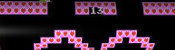
In Donald Michie's original tournament against MENACE, which lasted 220 games and 16 hours, MENACE drew consistently after 20 games.
)
Taken from Trial and error by Donald Michie [2]
)
Graph showing MENACE's performance in the original tournament. Edit: Added the redrawn graph on the left.
After a while, Michie tried playing some more unusual games. For a while he was able to defeat MENACE, but MENACE quickly learnt to stop losing. You can read more about the original MENACE in A matchbox game learning-machine by Martin Gardner [1] and Trial and error by Donald Michie [2].
You may like to experiment with different tactics against MENACE yourself.
Play against MENACE
I have written a JavaScript implemenation of MENACE for you to play against. The source code for this implementation is available on GitHub.
When playing this version of MENACE, the contents of the matchboxes are shown on the right hand side of the page. The numbers shown on the boxes show how many beads corresponding to that move remain in the box. The red numbers show which beads have been picked in the current game.
The initial numbers of beads in the boxes and the incentives can be adjusted by clicking Adjust MENACE's settings above the matchboxes. My version of MENACE starts with more beads in each box than the original MENACE to prevent the early boxes from running out of beads, causing MENACE to resign.
Additionally, next to the board, you can set MENACE to play against random, or a player 2 version of MENACE.
Edit: After hearing me do a lightning talk about MENACE at CCC, Oliver Child built a copy of MENACE. Here are some pictures he sent me:
)
)
)
Edit: Oliver has written about MENACE and the version he built in issue 03 of Chalkdust Magazine.
Edit: Inspired by Oliver, I have built my own MENACE. I took it to the MathsJam Conference 2016. It looks like this:
)
References
[2] Trial and error by Donald Michie. Penguin Science Survey, 1961.
(Click on one of these icons to react to this blog post)
You might also enjoy...


Comments
Comments in green were written by me. Comments in blue were not written by me.
This is very neat. I wonder how long it would take to use that many matches to get all those match boxes. ×15 ×16 ×9 ×5 ×5
Duke Nukem
"When playing against skilled players, it is possible that the first move box runs out of beads. In this case, MENACE should be reset with more beads in the earlier boxes to give it more time to learn before it starts resigning."
If someone were doing this, you could do this automatically to avoid the perception or temptation of the operator to help it along. Instead of "oh, it's dead, let's repopulate the boxes", you could just make it part of the inter-game cleanup, like a garbage collection routine. After all the bead deleting/adding whatever, but before the next game starts, look at all the boxes, make sure that each box contains at least one of each color. Now this weakens the learning algorithm moderately, but it guarantees that it will never get stuck.×3 ×7 ×3 ×4 ×4
If someone were doing this, you could do this automatically to avoid the perception or temptation of the operator to help it along. Instead of "oh, it's dead, let's repopulate the boxes", you could just make it part of the inter-game cleanup, like a garbage collection routine. After all the bead deleting/adding whatever, but before the next game starts, look at all the boxes, make sure that each box contains at least one of each color. Now this weakens the learning algorithm moderately, but it guarantees that it will never get stuck.
(anonymous)
@Matthew: Thank you for such a quick response. Just to let you know that that link did not work after .../tree/master/output, but I managed to search around for the right files :). In these files MENACE plays the Nought right? and the user plays the Cross?
×2 ×2 ×2 ×2 ×2
(anonymous)
@Finlay: You can find them at https://github.com/mscroggs/MENACE-pdf.... The files boxes0.pdf to boxes3.pdf are the boxes for a MENACE that plays first.×2 ×4 ×3 ×2 ×3
Matthew
Add a Comment
2015-03-25
This is an article which I wrote for the
first issue of
Chalkdust. I highly recommend reading the rest of the magazine (and trying
to solve the crossnumber I wrote for the issue).
In the classic arcade game Pac-Man, the player moves the title character through a maze. The aim of
the game is to eat all of the pac-dots that are spread throughout the maze while avoiding the ghosts
that prowl it.
While playing Pac-Man recently, my concentration drifted from the pac-dots and I began to think
about the best route I could take to complete the level.
Seven bridges of Königsberg
In the 1700s, Swiss mathematician Leonhard Euler studied a related problem. The city of
Königsberg had seven bridges, which the residents would try to cross while walking around the
town. However, they were unable to find a route crossing every bridge without repeating one of them.
)
Diagram showing the bridges in Königsberg. If you have not
seen this puzzle before, you may like to try to find a route crossing them all exactly once before reading on.
In fact, the city dwellers could not find such a route because it is impossible to do so, as
Euler proved in 1735. He first simplified the map of the city, by making the islands into vertices (or nodes)
and the bridges into edges.
)
A graph of the seven bridges problem.
This type of diagram has (slightly confusingly) become known as a graph, the study of which is
called graph theory. Euler represented Königsberg in this way as he realised that the shape of the
islands is irrelevant to the problem: representing the problem as a graph gets rid of this useless information
while keeping the important details of how the islands are connected.
Euler next noticed that if a route crossing all the bridges exactly once was possible then whenever
the walker took a bridge onto an island, they must take another bridge off the island. In this way,
the ends of the bridges at each island can be paired off. The only bridge ends that do not need a
pair are those at the start and end of the circuit.
This means that all of the vertices of the graph except two (the first and last in the route) must have an even number of edges connected to them; otherwise there is no route around the graph
travelling along each edge exactly once. In Königsberg, each island is connected to an odd number of bridges. Therefore the route that
the residents were looking for did not exist (a route now exists due to two of the bridges being destroyed during World War II).
This same idea can be applied to Pac-Man. By ignoring the parts of the maze without pac-dots the pac-graph
can be created, with the paths and the junctions forming the edges and vertices respectively. Once this
is done there will be twenty-four vertices, twenty of which will be connected to an odd number of edges, and so it is impossible to eat
all of the pac-dots without repeating some edges or travelling along parts of the maze with no pac-dots.
)
The Pac-graph. The odd nodes are shown in red.
This is a start, but it does not give us the shortest route we can take to eat all of the pac-dots: in
order to do this, we are going to have to look at the odd vertices in more detail.
The Chinese postman problem
The task of finding the shortest route covering all the edges of a graph has become known as the
Chinese postman problem as it is faced by postmen—they need to walk along each street to post
letters and want to minimise the time spent walking along roads twice—and it was first studied by
Chinese mathematician Kwan Mei-Ko.
As the seven bridges of Königsberg problem demonstrated, when trying to find a route, Pac-Man
will get stuck at the odd vertices. To prevent this from happening, all the vertices can be made into even
vertices by adding edges to the graph. Adding an edge to the graph corresponds to choosing an edge, or sequence
of edges, for Pac-Man to repeat or including a part of the maze without pac-dots. In order to complete the level
with the shortest distance travelled, Pac-Man wants to add the shortest total length of edges to the graph.
Therefore, in order to find the best route, Pac-Man must look at different ways to pair off the odd vertices and choose
the pairing which will add the least total distance to the graph.
The Chinese postman problem and the Pac-Man problem are slightly different: it is usually assumed
that the postman wants to finish where he started so he can return home. Pac-Man however can finish
the level wherever he likes but his starting point is fixed. Pac-Man may therefore leave one odd
node unpaired but must add an edge to make the starting node odd.
One way to find the required route is to look at all possible ways to pair up the odd vertices. With a low
number of odd vertices this method works fine, but as the number of odd vertices increases, the
method quickly becomes slower.
With four odd vertices, there are three possible pairings. For the Pac-Man problem there will be
over 13 billion (\(1.37\times 10^{10}\)) pairings to check. These pairings can be checked by a
laptop running overnight, but for not too many more vertices this method quickly becomes unfeasible.
With 46 odd nodes there will be more than one pairing per atom in the human body (\(2.53\times 10^{28}\)).
By 110 odd vertices there will be more pairings (\(3.47\times 10^{88}\)) than there are estimated to be atoms in the
universe. Even the greatest supercomputer will be unable to work its way through
all these combinations.
Better algorithms are known for this problem that reduce the amount of work on larger graphs. The number of
pairings to check in the method above increases like the factorial of the number of vertices. Algorithms are
known for which the amount of work to be done increases like a polynomial in the number of vertices. These algorithms
will become unfeasible at a much slower rate but will still be unable to deal with very large graphs.
Solution of the Pac-Man problem
For the Pac-Man problem, the shortest pairing of the odd vertices requires the edges marked in red to be
repeated. Any route which repeats these edges will be optimal. For example, the route in green will be
optimal.
)
)
One important element of the Pac-Man gameplay that I have neglected are the ghosts (Blinky, Pinky,
Inky and Clyde), which Pac-Man must avoid. There is a high chance that the ghosts will at some point
block the route shown above and ruin Pac-Man's optimality. However, any route repeating the red edges
will be optimal: at many junctions Pac-Man will have a choice of edges he could continue along. It may
be possible for a quick thinking player to utilise this freedom to avoid the ghosts and complete an optimal
game.
Additionally, the skilled player may choose when to take the edges that include the power pellets,
which allow Pac-Man to reverse the roles and eat the ghosts. Again cleverly timing these may allow
the player to complete an optimal route.
Unfortunately, as soon as the optimal route is completed, Pac-Man moves to the next level and the
player has to do it all over again ad infinitum.
A video
Since writing this piece, I have been playing Pac-Man using
MAME (Multiple Arcade Machine Emulator). Here is one game I played along
with the optimal edges to repeat for reference:
(Click on one of these icons to react to this blog post)
You might also enjoy...
Comments
Comments in green were written by me. Comments in blue were not written by me.
@William: You're right. In a number of places I could've turned round a few pixels earlier.
There seems to be no world record for just one Pac-Man level (and I don't have time to get good enough to speed run all 255 levels before it crashes!)×2 ×3 ×3 ×3 ×3
There seems to be no world record for just one Pac-Man level (and I don't have time to get good enough to speed run all 255 levels before it crashes!)
Matthew
This vid was billed as an "optimal" run but around 40 seconds in you eat one "pill" that you don't need to eat. Why don't you just speedrun the first level? This must have been done before. Can you beat the world record?×3 ×3 ×3 ×3 ×3
William
Add a Comment