Blog
2023-11-03
I showed off an unfinished version of the content in this blog post in the first
Finite Group live stream in October. I'll be showing off other upcoming things and other
content at future Finite Group events. If you'd like to watch this, you can sign up to our Patreon at
finitegroup.co.uk.
A few months ago at Cheltenham Science Festival, Hana Ayoob showed me how to make an 8-page zine.
If you've not make one before, I recommend following these steps now.
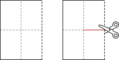
Take a piece of A4 paper, and fold it 3 times like this:
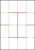
Unfold all the folds except the first one and cut along the red line:
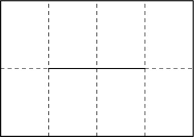
After unfolding, your paper should look like this:
Fold the paper in half the other way:
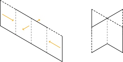
Push the two ends of the paper together so that the front of the middle bit of paper comes forward,
and the back goes backward:
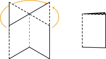
Finally, flatten all the pages and you have your zine:
You're now free to write or draw whatever you like on the 8 pages of your zine.
If you'd like to fold a zine that already has content printed on it, you can
print the instructions for the TMiP puzzle hunt that I wrote earlier this year, or you can print this blog post off in zine format.
A 16-page zine
If you're anything like me, you'll already be wondering if it's possible to do some more folding
and cutting to make a 16-page zine from a piece of A4. After some trial and error, I found that
you can if you fold the paper 4 times then cut along these red lines:
(This time, I've drawn the diagram with a portrait piece of paper, as this leads to a portrait zine. For an 8-page zine, a landscape piece of paper led to a portrait zine.)
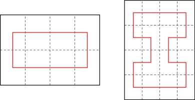
Instead of drawing which lines we need to cut, we can represent our two zines so far by drawing
lines that connect the pages in order:
During my experimentation, I saw that every second connection between pages must be horizontal.
These horizontal connections end up in the spine of the zine and allow the pages to turn.
If you can't visualise why the pages won't turn if this condition doesn't hold, try making a 16-page
zine like this:
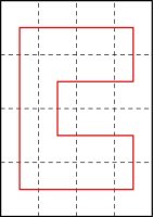
Now that we can make a 16-page zine, the obvious question is: can we make a 32-page zine?
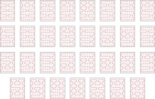
To answer this, we need to look for lines that go through all
32 pages where every second connection is a horizontal. I wrote a Python script to look for these and it
found 3:
The code also told me that the 8- and 16-page zines we know about are the only 8- and 16-page
zines. I'm only counting the zines where the pages in the final zine are portrait, and have the same side ratio a the original piece of A4 paper:
there will be other possible zines where the pages are landscape that we aren't counting.
2n-page zines
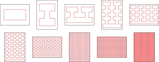
Now that we have 8-page, 16-page, and 32-page zines, we can look for patterns that we
can generalise to make a 2n-page zine. This generalisation was the first I
came up with:
There are, of course, many other generalisations that you could come up with.
How many zines?
While working towards our generalised zine, you may have started pondering another question:
for any given n, how many different 2n-page zines can be made?
For n=2, there's only one way to make a zine (fold the paper twice).
For n=3 to 6, we've already seen that there are 1, 1, and 3 ways to make zines. The code
I wrote was also able to tell me that there are 31 possible 64-page zines:
So the start of the sequence of the number of possible zines is: 1, 1, 1, 3, 31.
The number of different possible paths to check increases very quickly as we increase
n, so I was unable to compute the next term in a reasonable amount of time.
I've submitted this sequence to the OEIS. Let's
hope someone is able to work out the next term. If you're that someone, let me know!
(Click on one of these icons to react to this blog post)
You might also enjoy...
Comments
Comments in green were written by me. Comments in blue were not written by me.
Add a Comment
2023-09-02
This week, I've been at Talking Maths in Public (TMiP) in Newcastle. TMiP is a conference for anyone involved
in—or interested in getting involved in—any sort of maths outreach, enrichment, or public engagement activity. It was really good, and I highly recommend coming to TMiP 2025.
The Saturday morning at TMiP was filled with a choice of activities, including a puzzle hunt written by me: the Tyne trial.
At the start/end point of the Tyne trial, there was a locked box with a combination lock. In order to work out the combination for the lock, you needed to find some clues hidden around
Newcastle and solve a few puzzles.
Every team taking part was given a copy of these instructions.
Some people attended TMiP virtually, so I also made a version of the Tyne trial that included links to Google Street View and photos from which the necessary information could be obtained.
You can have a go at this at mscroggs.co.uk/tyne-trial/remote. For anyone who wants to try the puzzles without searching through virtual Newcastle,
the numbers that you needed to find are:
- Clue #1: \(a\) is 9.
- Clue #2: \(b\) is 5.
- Clue #3: \(c\) is 1838.
- Clue #4: \(d\) is 1931.
- Clue #5: \(e\) is 1619.
- Clue #6: \(f\) is 48.
- Clue #7: \(g\) is 1000.
The solutions to the puzzles and the final puzzle are below. If you want to try the puzzles for yourself, do that now before reading on.
Puzzle for clue #2: Palindromes
We are going to start with a number then repeat the following process: if the number you have is a palindrome, stop;
otherwise add the number to itself backwards.
For example, if we start with 219, then we do: $$219\xrightarrow{+912}1131\xrightarrow{+1311}2442.$$
If you start with the number \(10b+9\) (ie 59), what palindrome do you get?
(If you start with 196, it is unknown whether you will ever get a palindrome.)
Puzzle for clue #3: Mostly ones
There are 12 three-digit numbers whose digits are 1, 2, 3, 4, or 5 with exactly two digits that are ones.
How many \(c\)-digit (ie 1838-digit) numbers are there whose digits are 1, 2, 3, 4, or 5 with exactly \(c-1\) digits (ie 1837) that are ones?
Puzzle for clue #4: is it an integer?
The largest value of \(n\) such that \((n!-2)/(n-2)\) is an integer is 4. What is the largest value of \(n\) such that
\((n!-d)/(n-d)\) (ie \((n!-1931)/(n-1931)\)) is an integer?
Puzzle for clue #5: How many steps?
We are going to start with a number then repeat the following process:
if we've reached 0, stop; otherwise subtract the smallest prime factor of the current number.
For example, if we start with 9, then we do: $$9\xrightarrow{-3}6\xrightarrow{-2}4\xrightarrow{-2}2\xrightarrow{-2}0.$$ It took 4 steps to get to 0.
What is the smallest starting number such that this process will take \(e\) (ie 1619) steps?
Puzzle for clue #6: Four-digit number
I thought of a four digit number. I removed a
digit to make a three digit number, then added my two numbers together.
The result is \(200f+127\) (ie 9727). What was my original number?
Puzzle for clue #7: Dice
If you roll two six-sided fair dice, the most likely total is 7. What is the most likely total if you rolled \(1470+g\) (ie 2470) dice?
The final puzzle
The final puzzle involves using the answers to the five puzzles to find the four digit code that
opens the box (and the physical locked box that was in the library on
Saturday. To give hints to this code, each clue was given a "score".
The score of a number is the number of values of \(i\) such that the \(i\)th digit
of the code is a factor of the \(i\)th digit of the number.
For example, if the code was 1234, then the score of the number 3654 would be 3 (because
1 is a factor of 3; 2 is a factor of 6; and 4 is a factor of 4).
The seven clues to the final code are:
- Clue #1: 6561 scores 2 points.
- Clue #2: 1111 scores 0 points.
- Clue #3: 7352 scores 1 points.
- Clue #4: 3562 scores 1 points.
- Clue #5: 3238 scores 1 points.
- Clue #6: 8843 scores 1 points.
- Clue #7: 8645 scores 3 points.
(Click on one of these icons to react to this blog post)
You might also enjoy...
Comments
Comments in green were written by me. Comments in blue were not written by me.
Add a Comment
Image: Chalkdust Magazine
Chalkdust issue 17
2023-05-22
For the past couple of months, I've once again been spending an awful lot of my spare time working
on Chalkdust. Today you can see the result of all this hard work: Chalkdust issue 17.
I recommend checking out the entire magazine: you can read it online
or order a physical copy.
My most popular contribution to the magazine is probably the crossnumber.
I enjoyed writing this one; hope you enjoy solving it.
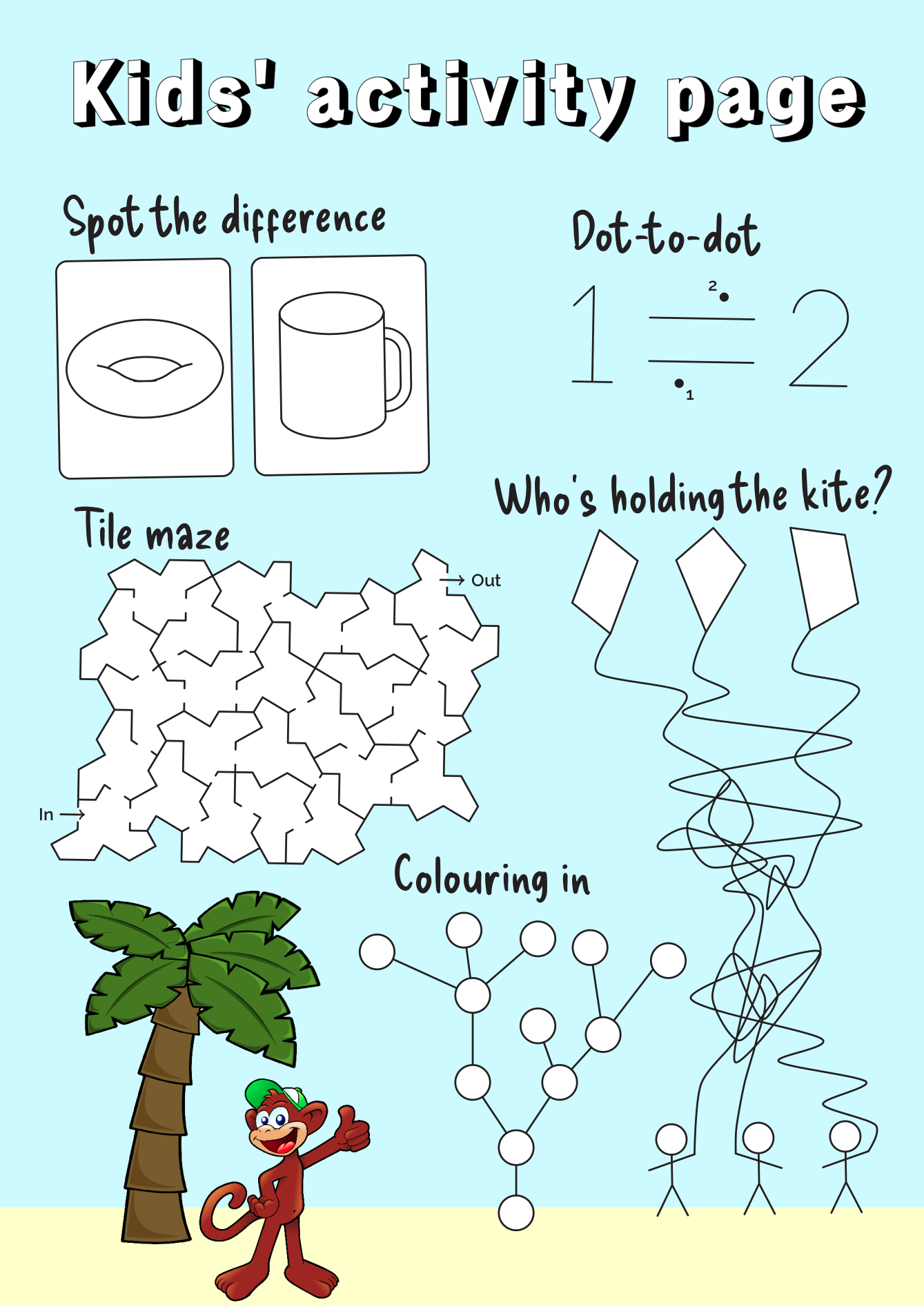
I also spent some time making this for the back page of the magazine. It's probably the most
fun I've had making something stupid for Chalkdust for ages.
Chalkdust Magazine
(Click on one of these icons to react to this blog post)
You might also enjoy...
Comments
Comments in green were written by me. Comments in blue were not written by me.
Add a Comment
2023-04-12
If, like me, you grew up in the 90s, then one of your earliest experiences of programming was
probably using Logo. In Logo, you use various commands to move a "turtle" around the screen. As the turtle moves,
it can draw lines. I have a very strong memory from early secondary school of spending a few maths
lessons in the computer room writing Logo programs to draw isometric houses.
If you read this blog regularly, you'll probably have noticed that I'm a fan of the game
Asteroids. Over the last few weeks, I've been working on Logo Asteroids,
a version of Asteroids where you control your spaceship using Logo commands. You can play this game
at mscroggs.co.uk/logo.
If you've not used Logo before, or if it's been so long since you have that you've forgotten the commands,
this blog post will guide you through how to get started. If you're confident in your Logo skills,
you might still want to scroll to the end of this post, where I share some custom Logo commands that you
might find helpful.
The game's source code is available on Github;
you can also use the GitHub issue tracker to report bugs and make feature requests.
Moving the turtle
If you're starting out in Logo, the first thing you'll want to do is move the turtle.
You can move it forwards or backwards using the commands fd or
bk followed by a number of pixels:
Logo
fd 100
bk 75
To change the direction in which the turtle is facing, you can use the command rt (right)
or lt (left) followed by an angle in degrees:
Logo
rt 90
lt 45
You can also chain together multiple commands on a single line like this:
Logo
fd 100 rt 90 fd 100 lt 90
By default, a line is drawn whenever the turtle moves forward or backwards. You can stop lines from being
drawn by running the command pu (pen up). To start drawing again, run
pd (pen down). If you want to make the game needlessly harder for yourself, you can use the command ht (hide turtle). To make the game easier again, run st (show turtle).
In a normal Logo program, the lines that you draw will stay there until you clear the screen (cs). In Logo Asteroids, the lines will only be visible for a limited amount
of time, and the asteroids will bounce off them while they are visible. To prevent too many lines from being drawn too quickly,
the turtle can move a maximum of 1000 pixels in a single command (or chain of commands).
Special commands for Logo Asteroids
As well as the Logo commands, there are some commands I have included that are specific to Logo
Asteroids. These are:
Logo
start
fire
help
The command start will start the game. You'll need to run this before you can run any other commands. You'll also need to run it to start the game again if you
run out of lives.
The command fire will fire at the asteroids. This command can be run
a maximum of 10 times by a single chain of commands.
The command help will show details of all the available commands below the game.
Defining your own subroutines
If you write some Logo commands that you want to use lots of times, use can use the to command to define a subroutine.
For example, the following code defined a command called square that will draw a square of side length 50.
Logo
to square fd 50 rt 90 fd 50 rt 90 fd 50 rt 90 fd 50 rt 90 end
The subroutine can then be used by running:
Logo
square
The square subroutine can be simplified by using the repeat command:
Logo
to square repeat 4 [fd 50 rt 90] end
... or it could be made to take a side length as input:
Logo
to square :side repeat 4 [fd :side rt 90] end
This updated version of the square subroutine can then be used by running:
Logo
square 50
square 100
square 125
Helpful subroutines for Logo Asteroids
To help you get going with Logo Asteroids, I've written a few subroutines that you might find helful. See if you
can work out what they do before running them.
Logo
to burst repeat 10 [fire rt 36] end
to protect pu fd 30 pd rt 135 repeat 4 [fd 30 * sqrt 2 rt 90] lt 135 pu bk 30 pd end
to multifire rt 10 repeat 10 [fire lt 2] rt 10 end
If you write your own helpful subroutine, share it in the comments below. You can put <logo> and </logo> HTML tags around your subroutine to make it display more nicely in your comment.
To end this blog post, here's one final subroutine for you to try out:
Logo
to house pu setxy 400 225 seth 0 pd lt 30 fd 40 lt 60 fd 40 lt 120 fd 40 lt 60 fd 40 rt 120 fd 50 rt 60 fd 40 rt 120 fd 50 setxy 400 + 20 * cos 30 155 rt 180 fd 50 setxy 400 - 50 * cos 30 160 pu setxy 400 + 20 * cos 30 155 pd setxy 400 + 40 * cos 30 165 pu setxy 400 225 lt 60 pd fd 50 rt 60 fd 50 rt 120 fd 50 pu rt 60 fd 20 pd lt 120 fd 20 rt 120 fd 10 rt 60 fd 20 rt 60 fd 50 pu rt 60 fd 10 pd rt 120 fd 50 ht end
(Click on one of these icons to react to this blog post)
You might also enjoy...
Comments
Comments in green were written by me. Comments in blue were not written by me.
Very cool! Here's a combination of your "burst" and "protect" subroutines:
to f pu sety 195 setx 390 pd repeat 10 [fire fd 20 rt 36] pu home end
Aaron
I didn't include this one in the blog post, but here's a bonus fun command:
to randwalk repeat 100 [rt random 360 fd 10] end
Matthew
Add a Comment
2023-03-14
A circle of radius \(r\) on a piece of paper can be thought of as a line through all the points on the paper that are a distance \(r\) from the centre of the circle.
The length of this line (ie the circumference) is \(2\pi r\).
Due to the curvature of the Earth, the line through all the points that are a distance \(r\) from where you are currently standing will be less than \(2\pi r\) (although you might
not notice the difference unless \(r\) is very big). The type of curvature that a sphere has is often called positive curvature.
It is also possible to create surfaces that have negative curvature; or surfaces where the length of the line through all the points that are a distance \(r\) from a point is more than \(2\pi r\).
These surfaces are called hyperbolic surfaces.
Hyperbolic surfaces
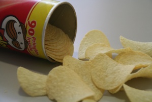
The most readily available example of a hyperbolic surface is a Pringle: Pringles are curved upwards in one direction, and curved downwards in the other direction.
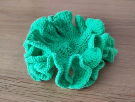
It's not immediately obvious what a larger hyperbolic surface would look like, but you can easily make one if you know how to crochet: simply increase the number of stitches at a
constant rate.
If it was possible to continue crocheting forever, you'd get an unbounded hyperbolic surface: the hyperbolic plane.
Over the last few weeks, I've been working on adding hyperbolic levels to Mathsteroids, the asteroids-inspired game that I started making levels for in 2018.
There are quite a few different ways to represent the hyperbolic plane in 2D. In this blog post we'll take a look at some of these; I encourage you to play the Mathsteroids level for each one as you
read so that you can get a feeling for their behaviour.
Poincaré disk
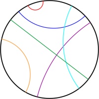
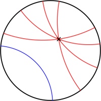
The Poincaré disk represents the hyperbolic plane as the interior of a circle. As objects move away from the centre of the circle, they appear smaller and smaller; and the circumference of
the circle is infinitely far from the centre of the circle. Straight lines on the hyperbolic plane appear on the Poincaré disk as either circles that meet the edge of the disk at right angles,
or straight lines through the centre of the circle.
One of the nicest properties of the Poincaré disk is that it correctly represents angles: If you measure the angle between to intersecting straight lines represented on the disk, then the value
you measure will be the same as the angles between the two lines in the actual hyperbolic plane.
This representation can be used to demonstrate some interesting properties of the hyperbolic plane.
In normal two dimensional space, if you are given a line and a point then there is exactly one line that goes through the point and is parallel to the first line.
But in hyperbolic space, there are many such parallel lines.
In Mathsteroids, there are two levels based on the Poincaré disk. The first level is bounded: you can only fly so far from the centre of the circle before
you hit the edge of the level and bounce back. (This prevents you from getting lost in the part of the disk where you would appear very very small.)
The second level is unbounded. In this level, you can fly as far as you like in any direction, but the point which is at the centre of the
disk will change when you go too far to prevent the ship from getting to small.
Beltrami–Klein disk
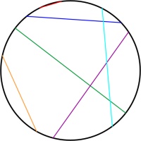
Simlar to the Poincaré disk, the Beltrami–Klein disk represents the hyperbolic plane using the interior of a circle, with the edge of the circle infinitely far away. Straight lines
in hyperbolic space will appear as straight lines in the Beltrami–Klein disk. The Beltrami–Klein disk is closely related to the Poincaré disk: the same line represented on both disks
will have its endpoints at the same points on the circle (although these endpoints are arguably not part of the line as they are on the circle that is infinitely far away).
Unlike in the Poincaré disk, angles are not correctly represented in the Beltrami–Klein disk. It can however be a very useful representation as straight lines appearing as straight lines
is a helpful feature.
Again, there are two Mathsteroids levels based on the Beltrami–Klein disk: a bounded level and an unbounded level.
Poincaré half-plane
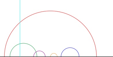
The Poincaré half-plane represents the hyperbolic plane using the half-plane above the \(x\)-axis. Straight lines in hyperbolic space are represented by either vertical
straight lines or semicircles with their endpoints on the \(x\)-axis.
Like the Poincaré disk, the Poincaré half-plane correctly represents the angles between lines.
There is one Mathsteroids level based on the Poincaré half-plane: this level is bounded so you can only travel so far away from where you start.
Band
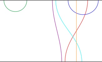
The band representation represents the hyperbolic plane as the strip between two horizontal lines. The strip extends forever to the left and right.
Straight lines on the band come in a variety of shapes.
There is one Mathsteroids level based on the band representation: the bounded level.
Hyperboloid and Gans plane
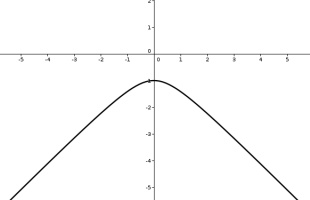
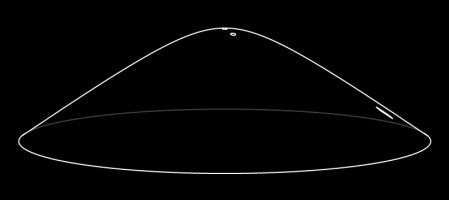
The hyperbolic plane can be represented on the surface of a hyperboloid. A hyperboloid is the shape you get if you rotate and hyperbola (a curve shaped like \(y=1/x\).)
Straight lines on this representation are the intersections of the hyperboloid with flat planes that go through the origin.
You can see what these straight lines look like by playing the (bounded) Mathsteroids level based on the hyperboloid.
The Gans plane is simply the hyperboloid viewed from above. There is a (bounded) Mathsteroids level based on the Gans plane.
(Click on one of these icons to react to this blog post)
You might also enjoy...
Comments
Comments in green were written by me. Comments in blue were not written by me.
Add a Comment


