
Blog
2022-12-29
This is the 100th blog post on this website!
But if I hadn't pointed this out,
you might not have noticed: the URL of the page is mscroggs.co.uk/blog/99 and not mscroggs.co.uk/blog/100.
This is a great example of an off-by-one error.
Off-by-one errors are one of the most common errors made when programming and elsewhere, and this is an excellent opportunity to blog about them.
Fence posts and fence panels
Imagine you want to make a straight fence that is 50m long. Each fencing panel is 2m long.
How many fence posts will you need?
Have a quick think about this before reading on.
If you're currently thinking about the number 25, then you've just made an off-by-one error.
The easiest way to see why is to think about some shorter fences.
If you want to make a fence that's 2m long, then you'll need just one fence panel. But one fence
post will not be enough: you'll need a second post to put at the other end of the fence panel.
If you want to make a 4m long fence, you'll need a post before the first panel, a post between
the two panels, and a post after the second panel: that's three posts in total.
In general, you'll always need one more fence post than panel, as you need a fence post
at the start of each panel and an extra post at the end of the final panel.
(Unless, of course, you're building a fence that is a closed loop.)
)
This fence has 4 fence panels but 5 fence posts
This fence post/fence panel issue appears surprisingly often, and can make counting things
quite difficult. For example, the first blog post
on this website was posted in 2012: ten years ago. But if you count the number of years listed in the
archive there are 11 years. If you release an issue of a magazine once a year, then issue 11 (not issue 10) will
be the issue released 10 years after you start not issue 10. If, like Chalkdust,
you release issues two times a year, issue 21 (not issue 20) will be the 10 year issue.
Half-open intervals
An interval is called closed if it includes its starting and ending point, and open if it
doesn't include them. A half-open interval includes one end point and not the other.
Using half-open intervals makes counting things less difficult: including one endpoint but not the other is a bit like ignoring
the final (or first) fence post so that there are the same number of post and panels.
In Python, the range function includes the first number but not the last
(this is the sensible choice as including the final number and not the first would be very confusing).
range(5, 8) includes the numbers 5, 6, and 7 (but not 8).
By excluding the final number, the number of numbers in a range
will be equal to the difference between the two input numbers.
Excluding the final item so that the number of items in a range is equal to the difference between the start and end is a great way to
reduce opportunities for off-by-one errors, and isn't too hard to get used to.
Why start at 0?
We've seen a couple of causes of off-by-one errors, but we've not yet seen why this page's URL
contains 99 rather than 100. This is because the numbering of blog posts started at zero.
But why is it a sensible choice to start at 0?
Using a half-open range, the first \(n\) numbers starting at 1 would be range(1, n + 1); the first \(n\) numbers starting at 0 on the other hand
would be range(0, n). The second option is neater, as you don't have to add one to the final number; the first option opens up more opportunities for
off-by-one errors.
This is one of the reasons why Python and many other programming languages start their numbering from 0.
Why doesn't everyone start at 0?
Starting at 0 and using half-open intervals to represent ranges of integers seem like good ways to help people avoid making off-by-one errors, but this choice is not perfect.
If you want to write a range of numbers from 1 to 8 inclusive using this convention, you would have to write range(1, 9):
forgetting to add one to the final number in this situation is another source of off-by-one errors.
It's also more natural to many people to start counting from 1, so some programming languages choose different conventions. The following table sums up the different possible
conventions, which desirable properties they have, and which languages use them.
| Convenction | Languages using this convention | Length of range is difference between endpoints | range(START, n) contains \(n\) numbers | range(START, n) contains START | range(START, n) contains \(n\) |
| START=0, range includes first endpoint only | Python, Javascript, PHP, Rust, C, C++ | ✓ | ✓ | ✓ | ✗ |
| START=0, range includes last endpoint only | ✓ | ✓ | ✗ | ✓ | |
| START=0, range includes both endpoints | ✗ | ✗ | ✓ | ✓ | |
| START=0, range includes neither endpoint | ✗ | ✗ | ✗ | ✗ | |
| START=1, range includes first endpoint only | ✓ | ✗ | ✓ | ✗ | |
| START=1, range includes last endpoint only | ✓ | ✗ | ✗ | ✓ | |
| START=1, range includes both endpoints | Matlab, Julia, Fortran | ✗ | ✓ | ✓ | ✓ |
| START=1, range includes neither endpoint | ✗ | ✗ | ✗ | ✗ |
(I don't know of any languages that use any of the other conventions, but if you have please let me know in the comments below and I'll add them.)
None of the conventions manages to remove all the possible sources of confusion, so it looks like off-by-one errors are here to stay.
(Click on one of these icons to react to this blog post)
You might also enjoy...


Comments
Comments in green were written by me. Comments in blue were not written by me.
Add a Comment
2020-02-04
This is the second post in a series of posts about my PhD thesis.
During my PhD, I spent a lot of time working on the open source boundary element method Python library Bempp.
The second chapter of my thesis looks at this software, and some of the work we did to improve its performance and to make solving problems with it more simple,
in more detail.
Discrete spaces
We begin by looking at the definitions of the discrete function spaces that we will use when performing discretisation. Imagine that the boundary of our region has been split into a mesh of triangles.
(The pictures in this post show a flat mesh of triangles, although in reality this mesh will usually be curved.)
We define the discrete spaces by defining a basis function of the space. The discrete space will have one of these basis functions for each triangle, for each edge, or for each vertex (or a combination
of these) and the space is defined to contain all the sums of multiples of these basis functions.
The first space we define is DP0 (discontinuous polynomials of degree 0). A basis function of this space has the value 1 inside one triangle, and has the value 0 elsewhere; it
looks like this:
)
Next we define the P1 (continuous polynomials of degree 1) space. A basis function of this space has the value 1 at one vertex in the mesh, 0 at every other vertex, and is linear inside
each triangle; it looks like this:
)
Higher degree polynomial spaces can be defined, but we do not use them here.
For Maxwell's equations, we need different basis functions, as the unknowns are vector functions. The two most commonly spaces are RT (Raviart–Thomas) and NC (Nédélec) spaces.
Example basis functions of these spaces look like this:
)
RT (left) and NC (right) basis functions.
Preconditioning
Suppose we are trying to solve \(\mathbf{A}\mathbf{x}=\mathbf{b}\), where \(\mathbf{A}\) is a matrix, \(\mathbf{b}\) is a (known) vector, and \(\mathbf{x}\) is the vector we are trying to find.
When \(\mathbf{A}\) is a very large matrix, it is common to only solve this approximately, and many methods are known that can achieve
good approximations of the solution. To get a good idea of how quickly these methods will work, we can calculate the condition number of the matrix: the condition number
is a value that is big when the matrix will be slow to solve (we call the matrix ill-conditioned); and is small when the matrix will be fast to solve (we call the matrix well-conditioned).
The matrices we get when using the boundary element method are often ill-conditioned. To speed up the solving process, it is common to use preconditioning: instead of solving \(\mathbf{A}\mathbf{x}=\mathbf{b}\), we can
instead pick a matrix \(\mathbf{P}\) and solve $$\mathbf{P}\mathbf{A}\mathbf{x}=\mathbf{P}\mathbf{b}.$$ If we choose the matrix \(\mathbf{P}\) carefully, we can obtain a matrix
\(\mathbf{P}\mathbf{A}\) that has a lower condition number than \(\mathbf{A}\), so this new system could
be quicker to solve.
When using the boundary element method, it is common to use properties of the Calderón projector to work out some good preconditioners.
For example, the single layer operator \(\mathsf{V}\) when discretised is often ill-conditioned, but the product of it and the hypersingular operator \(\mathsf{W}\mathsf{V}\) is often
better conditioned. This type of preconditioning is called operator preconditioning or Calderón preconditioning.
If the product \(\mathsf{W}\mathsf{V}\) is discretised, the result is $$\mathbf{W}\mathbf{M}^{-1}\mathbf{V},$$ where \(\mathbf{W}\) and \(\mathbf{V}\)
are discretisations of \(\mathsf{W}\) and \(\mathsf{V}\), and \(\mathbf{M}\) is a matrix
called the mass matrix that depends on the discretisation spaces used to discretise \(\mathsf{W}\) and \(\mathsf{V}\).
In our software Bempp, the mass matrices \(\mathbf{M}\) are automatically included in product like this, which makes using preconditioning like this easier to program.
As an alternative to operator preconditioning, a method called mass matrix preconditioning is often used: this method uses the inverse mass matrix \(\mathbf{M}^{-1}\) as a preconditioner (so is like the operator
preconditioning example without the \(\mathbf{W}\)).
More discrete spaces
As the inverse mass matrix \(\mathbf{M}^{-1}\) appears everywhere in the preconditioning methods we would like to use, it would be great if this matrix was well-conditioned: as if it is, it's inverse
can be very quickly and accurately approximated.
There is a condition called the inf-sup condition: if the inf-sup condition holds for the discretisation spaces used, then the mass matrix will be well-conditioned. Unfortunately, the inf-sup
condition does not hold when using a combination of DP0 and P1 spaces.
All is not lost, however, as there are spaces we can use that do satisfy the inf-sup condition. We call these DUAL0 and DUAL1, and they form inf-sup stable pairs with P1 and DP0 (respectively).
They are defined using the barycentric dual mesh: this mesh is defined by joining each point in a triangle with the midpoint of the opposite side, then making polygons with all the small triangles that
touch a vertex in the original mesh:
)
The mesh (left), the barycentric refinement (centre), and the dual grid (right)
Example DUAL1 and DUAL0 basis functions look like this:
)
DUAL1 (left) and DUAL0 (right) basis functions.
For Maxwell's equations, we define BC (Buffa–Christiansen) and RBC (rotated BC) functions to make inf-sup stable spaces pairs. Example BC and RBC basis functions look like this:
)
Example BC (left) and RBC (right) basis functions.
My thesis then gives some example Python scripts that show how these spaces can be used in Bempp to solve some example problems, concluding chapter 2 of my thesis.
Why not take a break and have a slice of the following figure before reading on.
)
An electromagnetic wave scattering off a perfectly conducting metal cake. This solution was found using a Calderón preconditioned boundary element method.
Previous post in series

This is the second post in a series of posts about my PhD thesis.
Next post in series

(Click on one of these icons to react to this blog post)
You might also enjoy...


Comments
Comments in green were written by me. Comments in blue were not written by me.
Add a Comment
2017-03-08
This post appeared in issue 05 of Chalkdust. I strongly
recommend reading the rest of Chalkdust.
Take a long strip of paper. Fold it in half in the same direction a few times. Unfold it and look at the shape the edge of the paper
makes. If you folded the paper \(n\) times, then the edge will make an order \(n\) dragon curve, so called because it faintly resembles a
dragon. Each of the curves shown on the cover of issue 05 of Chalkdust is an order 10 dragon
curve.
)
)
Top: Folding a strip of paper in half four times leads to an order four dragon curve (after rounding the corners). Bottom: A level 10 dragon curve resembling a dragon.
The dragon curves on the cover show that it is possible to tile the entire plane with copies of dragon curves of the same order. If any
readers are looking for an excellent way to tile a bathroom, I recommend getting some dragon curve-shaped tiles made.
An order \(n\) dragon curve can be made by joining two order \(n-1\) dragon curves with a 90° angle between their tails. Therefore, by
taking the cover's tiling of the plane with order 10 dragon curves, we may join them into pairs to get a tiling with order 11 dragon
curves. We could repeat this to get tilings with order 12, 13, and so on... If we were to repeat this ad infinitum we would arrive
at the conclusion that an order \(\infty\) dragon curve will cover the entire plane without crossing itself. In other words, an order
\(\infty\) dragon curve is a space-filling curve.
Like so many other interesting bits of recreational maths, dragon curves were popularised by Martin Gardner in one of his Mathematical Games columns in Scientific
American. In this column, it was noted that the endpoints of dragon curves of different orders (all starting at the same point) lie on
a logarithmic spiral. This can be seen in the diagram below.
)
The endpoints of dragon curves of order 1 to 10 with a logarithmic spiral passing through them.
Although many of their properties have been known for a long time and are well studied, dragon curves continue to appear in new and
interesting places. At last year's Maths Jam conference, Paul Taylor gave a talk about my favourite surprise occurrence of
a dragon.
Normally when we write numbers, we write them in base ten, with the digits in the number representing (from right to left) ones, tens,
hundreds, thousands, etc. Many readers will be familiar with binary numbers (base two), where the powers of two are used in the place of
powers of ten, so the digits represent ones, twos, fours, eights, etc.
In his talk, Paul suggested looking at numbers in base -1+i (where i is the square root of -1; you can find more adventures of i here) using the digits 0 and 1. From right to left, the columns of numbers in this
base have values 1, -1+i, -2i, 2+2i, -4, etc. The first 11 numbers in this base are shown below.
| Number in base -1+i | Complex number |
| 0 | 0 |
| 1 | 1 |
| 10 | -1+i |
| 11 | (-1+i)+(1)=i |
| 100 | -2i |
| 101 | (-2i)+(1)=1-2i |
| 110 | (-2i)+(-1+i)=-1-i |
| 111 | (-2i)+(-1+i)+(1)=-i |
| 1000 | 2+2i |
| 1001 | (2+2i)+(1)=3+2i |
| 1010 | (2+2i)+(-1+i)=1+3i |
Complex numbers are often drawn on an Argand diagram: the real part of the number is plotted on the horizontal axis and the imaginary part
on the vertical axis. The diagram to the left shows the numbers of ten digits or less in base -1+i on an Argand diagram. The points form
an order 10 dragon curve! In fact, plotting numbers of \(n\) digits or less will draw an order \(n\) dragon curve.
)
Numbers in base -1+i of ten digits or less plotted on an Argand diagram.
Brilliantly, we may now use known properties of dragon curves to discover properties of base -1+i. A level \(\infty\) dragon curve covers
the entire plane without intersecting itself: therefore every Gaussian integer (a number of the form \(a+\text{i} b\) where \(a\) and
\(b\) are integers) has a unique representation in base -1+i. The endpoints of dragon curves lie on a logarithmic spiral: therefore
numbers of the form \((-1+\text{i})^n\), where \(n\) is an integer, lie on a logarithmic spiral in the complex plane.
If you'd like to play with some dragon curves, you can download the Python code used
to make the pictures here.
(Click on one of these icons to react to this blog post)
You might also enjoy...
Comments
Comments in green were written by me. Comments in blue were not written by me.
Add a Comment
2016-10-08
During my Electromagnetic Field talk this year, I spoke about @mathslogicbot, my Twitter bot that is working its way through the tautologies in propositional calculus. My talk included my conjecture that the number of tautologies of length \(n\) is an increasing sequence (except when \(n=8\)). After my talk, Henry Segerman suggested that I also look at the number of contradictions of length \(n\) to look for insights.
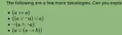
A contradiction is the opposite of a tautology: it is a formula that is False for every assignment of truth values to the variables. For example, here are a few contradictions:
$$\neg(a\leftrightarrow a)$$
$$\neg(a\rightarrow a)$$
$$(\neg a\wedge a)$$
$$(\neg a\leftrightarrow a)$$
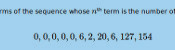
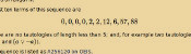
The first eleven terms of the sequence whose \(n\)th term is the number of contradictions of length \(n\) are:
$$0, 0, 0, 0, 0, 6, 2, 20, 6, 127, 154$$
This sequence is A277275 on OEIS. A list of contractions can be found here.
For the same reasons as the sequence of tautologies, I would expect this sequence to be increasing. Surprisingly, it is not increasing for small values of \(n\), but I again conjecture that it is increasing after a certain point.
Properties of the sequences
There are some properties of the two sequences that we can show. Let \(a(n)\) be the number of tautolgies of length \(n\) and let \(b(n)\) be the number of contradictions of length \(n\).
First, the number of tautologies and contradictions, \(a(n)+b(n)\), (A277276) is an increasing sequence. This is due to the facts that \(a(n+1)\geq b(n)\) and \(b(n+1)\geq a(n)\), as every tautology of length \(n\) becomes a contraction of length \(n+1\) by appending a \(\neg\) to be start and vice versa.
This implies that for each \(n\), at most one of \(a\) and \(b\) can be decreasing at \(n\), as if both were decreasing, then \(a+b\) would be decreasing. Sadly, this doesn't seem to give us a way to prove the conjectures, but it is a small amount of progress towards them.
(Click on one of these icons to react to this blog post)
You might also enjoy...

Comments
Comments in green were written by me. Comments in blue were not written by me.
Add a Comment
2016-10-06
Thanks to Marc, I noticed that today's date is a palindrome in two different date formats—DMMYY (61016) and DMMYYYY (6102016).
This made me wonder when there will be another date that is palindromic in multiple date formats, so I wrote a Python script to find out.
Turns out there's not too long to wait: 10 July 2017 will be palindromic in two date formats (MDDYY and MDDYYYY). But before that, there's 1 July 2017, which is palindromic in three date formats (YYMMD, YYMD and MDYY). Most exciting of all, however, is 2 February 2020, which is palindromic in 7 different formats!
The next palindromic dates are shown in the following table. It will update as the dates pass.
| \(n\) | Next day with \(\geq n\) palindromic formats | Formats |
| 1 | Today! | MDDYY |
| 2 | 2 May 2025 | YYMMD,YYMD,MDYY |
| 3 | 2 May 2025 | YYMMD,YYMD,MDYY |
| 4 | 2 March 2030 | YYYYMMDD,MMDDYYYY,YYYYMDD,MMDYY |
| 5 | 1 January 2110 | DDMYYYY,YYMDD,DDMYY,MMDYYYY,MMDYY |
| 6 | 1 January 2211 | YYMMD,DMYYYY,MDYYYY,YYMD,DMYY,MDYY |
A full list of future palindromic dates can be found here.
(Click on one of these icons to react to this blog post)
You might also enjoy...


Comments
Comments in green were written by me. Comments in blue were not written by me.
Add a Comment
Love your blog posts!
They make me get out of bed in the morning.
Just wanted to show my appreciation.
Cheers.