
Blog
PhD thesis, chapter 2
2020-02-04
This is the second post in a series of posts about my PhD thesis.
During my PhD, I spent a lot of time working on the open source boundary element method Python library Bempp.
The second chapter of my thesis looks at this software, and some of the work we did to improve its performance and to make solving problems with it more simple,
in more detail.
Discrete spaces
We begin by looking at the definitions of the discrete function spaces that we will use when performing discretisation. Imagine that the boundary of our region has been split into a mesh of triangles.
(The pictures in this post show a flat mesh of triangles, although in reality this mesh will usually be curved.)
We define the discrete spaces by defining a basis function of the space. The discrete space will have one of these basis functions for each triangle, for each edge, or for each vertex (or a combination
of these) and the space is defined to contain all the sums of multiples of these basis functions.
The first space we define is DP0 (discontinuous polynomials of degree 0). A basis function of this space has the value 1 inside one triangle, and has the value 0 elsewhere; it
looks like this:
)
Next we define the P1 (continuous polynomials of degree 1) space. A basis function of this space has the value 1 at one vertex in the mesh, 0 at every other vertex, and is linear inside
each triangle; it looks like this:
)
Higher degree polynomial spaces can be defined, but we do not use them here.
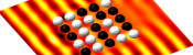
For Maxwell's equations, we need different basis functions, as the unknowns are vector functions. The two most commonly spaces are RT (Raviart–Thomas) and NC (Nédélec) spaces.
Example basis functions of these spaces look like this:
)
RT (left) and NC (right) basis functions.
Preconditioning
Suppose we are trying to solve \(\mathbf{A}\mathbf{x}=\mathbf{b}\), where \(\mathbf{A}\) is a matrix, \(\mathbf{b}\) is a (known) vector, and \(\mathbf{x}\) is the vector we are trying to find.
When \(\mathbf{A}\) is a very large matrix, it is common to only solve this approximately, and many methods are known that can achieve
good approximations of the solution. To get a good idea of how quickly these methods will work, we can calculate the condition number of the matrix: the condition number
is a value that is big when the matrix will be slow to solve (we call the matrix ill-conditioned); and is small when the matrix will be fast to solve (we call the matrix well-conditioned).
The matrices we get when using the boundary element method are often ill-conditioned. To speed up the solving process, it is common to use preconditioning: instead of solving \(\mathbf{A}\mathbf{x}=\mathbf{b}\), we can
instead pick a matrix \(\mathbf{P}\) and solve $$\mathbf{P}\mathbf{A}\mathbf{x}=\mathbf{P}\mathbf{b}.$$ If we choose the matrix \(\mathbf{P}\) carefully, we can obtain a matrix
\(\mathbf{P}\mathbf{A}\) that has a lower condition number than \(\mathbf{A}\), so this new system could
be quicker to solve.
When using the boundary element method, it is common to use properties of the Calderón projector to work out some good preconditioners.
For example, the single layer operator \(\mathsf{V}\) when discretised is often ill-conditioned, but the product of it and the hypersingular operator \(\mathsf{W}\mathsf{V}\) is often
better conditioned. This type of preconditioning is called operator preconditioning or Calderón preconditioning.
If the product \(\mathsf{W}\mathsf{V}\) is discretised, the result is $$\mathbf{W}\mathbf{M}^{-1}\mathbf{V},$$ where \(\mathbf{W}\) and \(\mathbf{V}\)
are discretisations of \(\mathsf{W}\) and \(\mathsf{V}\), and \(\mathbf{M}\) is a matrix
called the mass matrix that depends on the discretisation spaces used to discretise \(\mathsf{W}\) and \(\mathsf{V}\).
In our software Bempp, the mass matrices \(\mathbf{M}\) are automatically included in product like this, which makes using preconditioning like this easier to program.
As an alternative to operator preconditioning, a method called mass matrix preconditioning is often used: this method uses the inverse mass matrix \(\mathbf{M}^{-1}\) as a preconditioner (so is like the operator
preconditioning example without the \(\mathbf{W}\)).
More discrete spaces
As the inverse mass matrix \(\mathbf{M}^{-1}\) appears everywhere in the preconditioning methods we would like to use, it would be great if this matrix was well-conditioned: as if it is, it's inverse
can be very quickly and accurately approximated.
There is a condition called the inf-sup condition: if the inf-sup condition holds for the discretisation spaces used, then the mass matrix will be well-conditioned. Unfortunately, the inf-sup
condition does not hold when using a combination of DP0 and P1 spaces.
All is not lost, however, as there are spaces we can use that do satisfy the inf-sup condition. We call these DUAL0 and DUAL1, and they form inf-sup stable pairs with P1 and DP0 (respectively).
They are defined using the barycentric dual mesh: this mesh is defined by joining each point in a triangle with the midpoint of the opposite side, then making polygons with all the small triangles that
touch a vertex in the original mesh:
)
The mesh (left), the barycentric refinement (centre), and the dual grid (right)
Example DUAL1 and DUAL0 basis functions look like this:
)
DUAL1 (left) and DUAL0 (right) basis functions.
For Maxwell's equations, we define BC (Buffa–Christiansen) and RBC (rotated BC) functions to make inf-sup stable spaces pairs. Example BC and RBC basis functions look like this:
)
Example BC (left) and RBC (right) basis functions.
My thesis then gives some example Python scripts that show how these spaces can be used in Bempp to solve some example problems, concluding chapter 2 of my thesis.
Why not take a break and have a slice of the following figure before reading on.
)
An electromagnetic wave scattering off a perfectly conducting metal cake. This solution was found using a Calderón preconditioned boundary element method.
Previous post in series

This is the second post in a series of posts about my PhD thesis.
Next post in series

(Click on one of these icons to react to this blog post)
You might also enjoy...


Comments
Comments in green were written by me. Comments in blue were not written by me.
Add a Comment